User:Geek3/VectorFieldPlot

Field of a ring magnet, generated with VFPt

VectorFieldPlot (VFPt) is a python script that creates high quality fieldline plots in the svg vectorgraphics format.

About VectorFieldPlot

VectorFieldPlot was specially designed for the use in Wikimedia Commons. The lack of physical correct high-quality fieldplots in Wikimedia Commons has inspired me to compensate for this and provide a tool that enables users to create fieldplots as they require. VectorFieldPlot has grown beyond the stage of a small simple script that might already perform the task of creating plots of physical fields. Instead, it tries to fulfill its requirements the best way possible, which are namely:

• physical correctness / accuracy
• small file size / rendering efficiency
• image clarity and beauty
• image reusability

Other aspects are only of secondary order. VectorFieldPlot will not perform best at:

• code simplicity
• easy usage
• execution speed
• fancy graphical effects

Code

VectorFieldPlot is written in python3 and uses many features of SciPy as well as lxml. It can be directly executed after you inserted the description of your image at the end of the program code.

source code (2434 lines)

#!/usr/bin/python3 # -*- coding: utf8 -*- ''' VectorFieldPlot - plots electric and magnetic fieldlines in svg https://commons.wikimedia.org/wiki/User:Geek3/VectorFieldPlot Copyright (C) 2010-2023 Geek3 This program is free software; you can redistribute it and/or modify it under the terms of the GNU General Public License as published by the Free Software Foundation; either version 3 of the License, or (at your option) any later version. This program is distributed in the hope that it will be useful, but WITHOUT ANY WARRANTY; without even the implied warranty of MERCHANTABILITY or FITNESS FOR A PARTICULAR PURPOSE. See the GNU General Public License for more details. You should have received a copy of the GNU General Public License along with this program; if not, see https://www.gnu.org/licenses/ ''' version = '3.4' from math import * from lxml import etree from matplotlib import colors import base64 import numpy as np from numpy import array from scipy import integrate, interpolate, optimize, special import traceback # some helper functions def vabs(x): ''' vector norm of 2D vector. Note that scipy.linalg.norm is much slower ''' return hypot(x[0], x[1]) def vnorm(x): ''' vector normalisation ''' d = hypot(x[0], x[1]) if d != 0.: return array((x[0] / d, x[1] / d)) return array(x) def rot(xy, phi): ''' 2D vector rotation, counterclockwise ''' s, c = sin(phi), cos(phi) return array((c * xy[0] - s * xy[1], c * xy[1] + s * xy[0])) def cosv(v1, v2): ''' find the cosine of the angle between two vectors ''' dd = hypot(v1[0], v1[1]) * hypot(v2[0], v2[1]) if dd == 0.: return 1. cv = (v1[0] * v2[0] + v1[1] * v2[1]) / dd if cv >= 1.: return 1. elif cv <= -1.: return -1. return cv def sinv(v1, v2): ''' find the sine of the angle between two vectors ''' dd = hypot(v1[0], v1[1]) * hypot(v2[0], v2[1]) if dd == 0.: return 1. sv = (v1[0] * v2[1] - v1[1] * v2[0]) / dd if sv >= 1.: return 1. elif sv <= -1.: return -1. return sv def angle_dif(a1, a2): return ((a2 - a1 + pi) % (2. * pi)) - pi def cel(kc, p, a, b): """ Bulirsch complete elliptic integral, www.doi.org/10.1007/BF02165405 Despite implemented in slow Python, this is still faster than numerical integration or ellippi from mpmath """ if kc == 0.: return nan tol = 1e-9 # actual relative error will be tol**2 k = kc = fabs(kc) m = 1. if p > 0.: p = sqrt(p) b /= p else: f = kc * kc g = 1. - p q = (1. - f) * (b - a * p) f -= p p = sqrt(f / g) a = (a - b) / g b = a * p - q / (g * g * p) i = 0 while True: f = a a += b / p g = k / p b = 2. * (b + f * g) p += g g = m m += kc if fabs(g - kc) <= g * tol or i >= 10: break i += 1 kc = 2. * sqrt(k) k = kc * m return pi * .5 * (a * m + b) / (m * (m + p)) def list_interpolate(l, t): if t < l[0]: idx, frac = 0, 0. elif t > l[-1]: idx, frac = len(l) - 1, 0. else: n = interpolate.interp1d(l, range(len(l)), kind='linear')(t) idx = int(floor(n)) frac = n - idx if idx > 0 and idx >= len(l) - 1: idx, frac = len(l) - 2, frac + idx - (len(l) - 2) return idx, frac def pretty_vec(p): return ','.join(['{0:> 9.5f}'.format(i) for i in p]) class FieldplotDocument: ''' creates a svg document structure using lxml.etree ''' def __init__(self, name, width=800, height=600, digits=None, unit=100, center=None, licence='cc-by-sa', commons=False, bg_color='#ffffff'): self.name = name self.width = float(width) self.height = float(height) self.unit = float(unit) self.licence = licence self.commons = commons if digits is None: self.digits = max(0, 1.8 + log10(self.unit)) else: self.digits = float(digits) if center is None: self.center = [width / 2., height / 2.] else: self.center = [float(i) for i in center] # create document structure self.svg = etree.Element('svg', nsmap={None: 'http://www.w3.org/2000/svg', 'xlink': 'http://www.w3.org/1999/xlink'}) self.svg.set('version', '1.1') self.svg.set('baseProfile', 'full') self.svg.set('width', str(int(width))) self.svg.set('height', str(int(height))) # title self.title = etree.SubElement(self.svg, 'title') self.title.text = self.name # description self.desc = etree.SubElement(self.svg, 'desc') self.desc.text = '' self.desc.text += self.name + '\n' self.desc.text += 'created with VectorFieldPlot ' + version + '\n' self.desc.text += 'https://commons.wikimedia.org/wiki/User:Geek3/VectorFieldPlot\n' if commons: self.desc.text += """ about: https://commons.wikimedia.org/wiki/File:{0}.svg """.format(self.name) if self.licence == 'cc-by-sa': self.desc.text += """rights: Creative Commons Attribution ShareAlike 4.0\n""" self.desc.text += ' ' # background if bg_color is not None: self.background = etree.SubElement(self.svg, 'rect') self.background.set('id', 'background') self.background.set('x', '0') self.background.set('y', '0') self.background.set('width', str(width)) self.background.set('height', str(height)) self.background.set('fill', bg_color) # image elements self.content = etree.SubElement(self.svg, 'g') self.content.set('id', 'image') self.content.set('transform', 'translate({0},{1}) scale({2},-{2})'.format( self.center[0], self.center[1], self.unit)) self.content.set('clip-path', self._check_clip()) self.arrow_geo = {'x_nock':0.3,'x_head':3.8,'x_tail':-2.2,'width':4.5} # colormap similar to YlGnBu, but starting with white. cmap_WtGnBu = colors.LinearSegmentedColormap.from_list( 'WtGnBu', ((1.0, 1.0, 1.0), (0.929, 0.973, 0.694), (0.780, 0.914, 0.706), (0.498, 0.804, 0.733), (0.255, 0.714, 0.769), (0.114, 0.569, 0.753), (0.133, 0.369, 0.659), (0.145, 0.204, 0.580), (0.031, 0.114, 0.345)), 256) # colormap from aqua through yellow to fuchsia cmap_AqYlFs = colors.ListedColormap([np.clip((2*x, 2*(1-x), 4*(x-0.5)**2), 0, 1) for x in np.linspace(0., 1., 2049)]) cmap_AqYlFs_cyclic = colors.ListedColormap([np.clip( (fabs(1.5-fabs(3*x-2)), fabs(1.5-fabs(3*x-1)), 9*(x-0.5)**2), 0, 1) for x in np.linspace(0., 1., 3073)]) def _get_defs(self): if 'defs' not in dir(self): self.defs = etree.Element('defs') self.desc.addnext(self.defs) return self.defs def _check_fieldlines(self, linecolor='#000000', linewidth=1.): if 'fieldlines' not in dir(self): self.fieldlines = etree.SubElement(self.content, 'g') self.fieldlines.set('id', 'fieldlines') self.fieldlines.set('fill', 'none') self.fieldlines.set('stroke', linecolor) self.fieldlines.set('stroke-width', str(linewidth / self.unit)) self.fieldlines.set('stroke-linejoin', 'round') self.fieldlines.set('stroke-linecap', 'round') if 'count_fieldlines' not in dir(self): self.count_fieldlines = 0 def _check_symbols(self, bg=False): if 'count_symbols' not in dir(self): self.count_symbols = 0 if bg: if 'symbols_bg' not in dir(self): self.symbols_bg = etree.SubElement(self.content, 'g') self.symbols_bg.set('id', 'symbols_bg') return self.symbols_bg else: if 'symbols' not in dir(self): self.symbols = etree.SubElement(self.content, 'g') self.symbols.set('id', 'symbols') return self.symbols def _check_whitespot(self): if 'whitespot' not in dir(self): self.whitespot = etree.SubElement( self._get_defs(), 'radialGradient') self.whitespot.set('id', 'white_spot') for attr, val in [['cx', '0.65'], ['cy', '0.7'], ['r', '0.75']]: self.whitespot.set(attr, val) for col, of, opa in [['#ffffff', '0', '0.7'], ['#ffffff', '0.1', '0.5'], ['#ffffff', '0.6', '0'], ['#000000', '0.6', '0'], ['#000000', '0.75', '0.05'], ['#000000', '0.85', '0.15'], ['#000000', '1', '0.5']]: stop = etree.SubElement(self.whitespot, 'stop') stop.set('stop-color', col) stop.set('offset', of) stop.set('stop-opacity', opa) def _check_whitegradient(self): if 'whitegradient' not in dir(self): self.whitegradient = etree.SubElement( self._get_defs(), 'linearGradient') self.whitegradient.set('id', 'white_gradient') for attr, val in [['x1', '0.2'], ['x2', '0.8'], ['y1', '1.1'], ['y2', '-0.1']]: self.whitegradient.set(attr, val) for col, of, opa in [ ['#ffffff', '0', '0.5'], ['#ffffff', '0.3', '0.1'], ['#ffffff', '0.4', '0.3'], ['#ffffff', '0.6', '0.0'], ['#ffffff', '1.0', '0.6']]: stop = etree.SubElement(self.whitegradient, 'stop') stop.set('stop-color', col) stop.set('offset', of) stop.set('stop-opacity', opa) def _check_clip(self): if 'clip' not in dir(self): self.clip = etree.SubElement(self._get_defs(), 'clipPath') self.clip.set('id', 'image_clip') rect = etree.SubElement(self.clip, 'rect') rect.set('x', str(-self.center[0] / self.unit)) rect.set('y', str((self.center[1] - self.height) / self.unit)) rect.set('width', str(self.width / self.unit)) rect.set('height', str(self.height / self.unit)) return 'url(#image_clip)' def _get_arrowname(self, fillcolor='#000000'): if 'arrows' not in dir(self): self.arrows = {} if fillcolor not in self.arrows.keys(): arrow = etree.SubElement(self._get_defs(), 'path') self.arrows[fillcolor] = arrow arrow.set('id', 'arrow' + str(len(self.arrows))) arrow.set('stroke', 'none') arrow.set('fill', fillcolor) arrow.set('transform', 'scale({0})'.format(1. / self.unit)) arrow.set('d', 'M {0},0 L {1},{3} L {2},0 L {1},-{3} L {0},0 Z'.format( self.arrow_geo['x_nock'], self.arrow_geo['x_tail'], self.arrow_geo['x_head'], self.arrow_geo['width'] / 2.)) return self.arrows[fillcolor].get('id') def draw_charges(self, field, scale=1., bg=False): if scale == 0.0: return charges = [par for el, par in field.elements if el == 'monopole'] if len(charges) == 0: return symb = self._check_symbols(bg) self._check_whitespot() for charge in charges: c_group = etree.SubElement(symb, 'g') self.count_symbols += 1 c_group.set('id', 'charge{0}'.format(self.count_symbols)) c_group.set('transform', 'translate({0},{1}) scale({2},{2})'.format( charge['x'], charge['y'], scale / self.unit)) #### charge drawing #### c_bg = etree.SubElement(c_group, 'circle') c_shade = etree.SubElement(c_group, 'circle') c_symb = etree.SubElement(c_group, 'path') if charge['Q'] >= 0.: c_bg.set('style', 'fill:#ff0000; stroke:none') else: c_bg.set('style', 'fill:#3350ff; stroke:none') for attr, val in [['cx', '0'], ['cy', '0'], ['r', '14']]: c_bg.set(attr, val) c_shade.set(attr, val) c_shade.set('style', 'fill:url(#white_spot); stroke:#000000; stroke-width:2') # plus sign if charge['Q'] >= 0.: c_symb.set('d', 'M 2,2 V 8 H -2 V 2 H -8 V -2' + ' H -2 V -8 H 2 V -2 H 8 V 2 H 2 Z') # minus sign else: c_symb.set('d', 'M 8,2 H -8 V -2 H 8 V 2 Z') c_symb.set('style', 'fill:#000000; stroke:none') def draw_dipoles(self, field, scale=1., bg=False): dipoles = [par for el, par in field.elements if el == 'dipole'] if len(dipoles) == 0: return symb = self._check_symbols(bg) self._check_whitespot() for dipole in dipoles: x, y, px, py = [dipole[k] for k in ['x', 'y', 'px', 'py']] d_group = etree.SubElement(symb, 'g') self.count_symbols += 1 d_group.set('id', 'dipole{0}'.format(self.count_symbols)) d_group.set('transform', 'translate({0},{1}) scale({2},{2})'.format( x, y, scale / self.unit)) #### dipole drawing #### d_bg = etree.SubElement(d_group, 'circle') d_shade = etree.SubElement(d_group, 'circle') d_symb = etree.SubElement(d_group, 'path') d_bg.set('style', 'fill:#aaaaaa; stroke:none') for attr, val in [['cx', '0'], ['cy', '0'], ['r', '14']]: d_bg.set(attr, val) d_shade.set(attr, val) d_shade.set('style', 'fill:url(#white_spot); stroke:#000000; stroke-width:2') # arrow d_symb.set('d', 'M -8,2 H 0 V 8 L 10,0 L 0,-8 V -2 H -8 V 2 Z') d_symb.set('style', 'fill:#000000; stroke:none') if py != 0: d_symb.set('transform', 'rotate({:.5f})'.format(degrees(atan2(py, px)))) def draw_charged_wires(self, field, scale=1., bg=False): wires = [par for el, par in field.elements if el == 'charged_wire'] if len(wires) == 0: return symb = self._check_symbols(bg) self._check_whitegradient() for wire in wires: c_group = etree.SubElement(symb, 'g') self.count_symbols += 1 c_group.set('id', 'wire{0}'.format(self.count_symbols)) c_group.set('transform', 'translate({0},{1}) scale({2},{2})'.format( wire['x'], wire['y'], scale / self.unit)) #### wire drawing #### c_bg = etree.SubElement(c_group, 'circle') c_shade = etree.SubElement(c_group, 'circle') c_symb = etree.SubElement(c_group, 'path') for attr, val in [['cx', '0'], ['cy', '0'], ['r', '14']]: c_bg.set(attr, val) c_shade.set(attr, val) c_shade.set('style', 'fill:url(#white_gradient); stroke:#000000; stroke-width:2') # plus sign if wire['q'] >= 0.: c_symb.set('d', 'M 2,2 V 8 H -2 V 2 H -8 V -2' + ' H -2 V -8 H 2 V -2 H 8 V 2 H 2 Z') c_bg.set('style', 'fill:#ff0000; stroke:none') # minus sign else: c_symb.set('d', 'M 8,2 H -8 V -2 H 8 V 2 Z') c_bg.set('style', 'fill:#3350ff; stroke:none') c_symb.set('style', 'fill:#000000; stroke:none') def draw_currents(self, field, scale=1., bg=False): wires = [par for el, par in field.elements if el == 'wire'] ringcurrents = [par for el, par in field.elements if el == 'ringcurrent'] if len(wires) + len(ringcurrents) == 0: return symb = self._check_symbols(bg) self._check_whitespot() currents = [] for w in wires: currents.append(w) for cur in ringcurrents: x0, y0 = array([cur['x'], cur['y']]) + rot([0., cur['R']], cur['phi']) x1, y1 = array([cur['x'], cur['y']]) - rot([0., cur['R']], cur['phi']) currents.append({'x':x0, 'y':y0, 'I':cur['I']}) currents.append({'x':x1, 'y':y1, 'I':-cur['I']}) for cur in currents: c_group = etree.SubElement(symb, 'g') self.count_symbols += 1 if cur['I'] >= 0.: direction = 'out' else: direction = 'in' c_group.set('id', 'current_{0}{1}'.format(direction, self.count_symbols)) c_group.set('transform', 'translate({0},{1}) scale({2},{2})'.format( cur['x'], cur['y'], scale / self.unit)) #### current drawing #### c_bg = etree.SubElement(c_group, 'circle') c_shade = etree.SubElement(c_group, 'circle') c_bg.set('style', 'fill:#b0b0b0; stroke:none') for attr, val in [['cx', '0'], ['cy', '0'], ['r', '14']]: c_bg.set(attr, val) c_shade.set(attr, val) c_shade.set('style', 'fill:url(#white_spot); stroke:#000000; stroke-width:2') if cur['I'] >= 0.: # dot c_symb = etree.SubElement(c_group, 'circle') c_symb.set('cx', '0') c_symb.set('cy', '0') c_symb.set('r', '4') else: # cross c_symb = etree.SubElement(c_group, 'path') c_symb.set('d', 'M {1},-{0} L {0},-{1} L {2},{3} L {0},{1} \ L {1},{0} {3},{2} L -{1},{0} L -{0},{1} L -{2},{3} L -{0},-{1} L -{1},-{0} \ L {3},-{2} L {1},-{0} Z'.format(11.1, 8.5, 2.6, 0)) c_symb.set('style', 'fill:#000000; stroke:none') def draw_magnets(self, field, bg=False, linewidth=4): coils = [par for el, par in field.elements if el == 'coil'] if len(coils) == 0: return symb = self._check_symbols(bg) for coil in coils: m_group = etree.SubElement(symb, 'g') self.count_symbols += 1 m_group.set('id', 'magnet{0}'.format(self.count_symbols)) m_group.set('transform', 'translate({0},{1}) rotate({2})'.format( coil['x'], coil['y'], degrees(coil['phi']))) #### magnet drawing #### r = coil['R']; l = coil['Lhalf'] colors = ['#00cc00', '#ff0000'] SN = ['S', 'N'] if coil['I'] < 0.: colors.reverse() SN.reverse() m_defs = etree.SubElement(m_group, 'defs') m_gradient = etree.SubElement(m_defs, 'linearGradient') m_gradient.set('id', 'magnetGrad{0}'.format(self.count_symbols)) for attr, val in [['x1', '0'], ['x2', '0'], ['y1', str(coil['R'])], ['y2', str(-coil['R'])], ['gradientUnits', 'userSpaceOnUse']]: m_gradient.set(attr, val) for col, of, opa in [['#000000', '0', '0.125'], ['#ffffff', '0.07', '0.125'], ['#ffffff', '0.25', '0.5'], ['#ffffff', '0.6', '0.2'], ['#000000', '1', '0.33']]: stop = etree.SubElement(m_gradient, 'stop') stop.set('stop-color', col) stop.set('offset', of) stop.set('stop-opacity', opa) for i in [0, 1]: rect = etree.SubElement(m_group, 'rect') for attr, val in [['x', [-l, 0][i]], ['y', -r], ['width', [2*l, l][i]], ['height', 2 * r], ['style', 'fill:{0}; stroke:none'.format(colors[i])]]: rect.set(attr, str(val)) rect = etree.SubElement(m_group, 'rect') for attr, val in [['x', -l], ['y', -r], ['width', 2 * l], ['height', 2 * r], ['style', 'fill:url(#magnetGrad{0}); stroke-width:{1}; stroke-linejoin:miter; stroke:#000000'.format(self.count_symbols, linewidth / self.unit)]]: rect.set(attr, str(val)) rot = round(degrees(-coil['phi']) / 90.) * 90. x = max(0.5, min(0.5 * l * 0.75 / r, 0.65)) for i in [0, 1]: text = etree.SubElement(m_group, 'text') lr = min(r, 0.75 * l) for attr, val in [['text-anchor', 'middle'], ['y', -r], ['transform', 'translate({0},0) rotate({3}) translate(0,{1}) scale({2},-{2})'.format( [-x, x][i] * l, -0.44 * lr, lr / 100., rot)], ['style', 'fill:#000000; stroke:none; ' + 'font-size:120px; font-family:Bitstream Vera Sans']]: text.set(attr, str(val)) text.text = SN[i] def draw_line(self, fieldline, maxdist=10., linewidth=2., linecolor='#000000', attributes={}, arrows_style=None): ''' draws a calculated fieldline from a FieldLine object to the FieldplotDocument svg image ''' self._check_fieldlines(linecolor, linewidth) self.count_fieldlines += 1 bounds = {} bounds['x0'] = -(self.center[0] + 0.5 * linewidth) / self.unit bounds['y0'] = -(self.height - self.center[1] + 0.5 * linewidth) / self.unit bounds['x1'] = (self.width - self.center[0] + 0.5 * linewidth) / self.unit bounds['y1'] = (self.center[1] + 0.5 * linewidth) / self.unit # fetch the polyline from the fieldline object polylines = fieldline.get_polylines(self.digits, maxdist, bounds) if len(polylines) == 0: return line = etree.Element('path') if self.fieldlines.get('stroke') != linecolor: line.set('stroke', linecolor) if self.fieldlines.get('stroke-width') != str(linewidth / self.unit): line.set('stroke-width', str(linewidth / self.unit)) for attr, val in attributes.items(): line.set(attr, val) #### line drawing #### path_data = [] for polyline in polylines: line_points = polyline['path'] for i, p in enumerate(line_points): # go through all points, draw them if line segment is visible ptext = '{1:.{0}f},{2:.{0}f}'.format( int(ceil(self.digits)), p[0], p[1]) if i == 0: path_data.append('M ' + ptext) else: path_data.append('L ' + ptext) # close path if possible if (vabs(polylines[0]['path'][0] - polylines[-1]['path'][-1]) < .1**self.digits): closed = True if len(polylines) == 1: path_data.append('Z') elif len(polylines) > 1: # rearrange array cyclic path_data.pop(0) while path_data[0][0] != 'M': path_data.append(path_data.pop(0)) else: closed = False path = ' '.join(path_data) line.set('d', path) if arrows_style is None: # include path directly into document structure line.set('id', 'fieldline{0}'.format(self.count_fieldlines)) self.fieldlines.append(line) else: line_and_arrows = etree.SubElement(self.fieldlines, 'g') line_and_arrows.set('id', 'fieldline' + str(self.count_fieldlines)) line_and_arrows.append(line) line_and_arrows.append(self._draw_arrows(arrows_style, linewidth, polylines, fieldline, linecolor, closed)) def _draw_arrows(self, arrows_style, linewidth, polylines, fieldline, linecolor='#000000', closed=False): ''' draws arrows on polylines. options in "arrows_style": min_arrows: minimum number of arrows per segment max_arrows: maximum number of arrows per segment (None: no limit) dist: optimum distance between arrows scale: relative size of arrows to linewidth offsets {'start', 'end', 'leave_image', 'enter_image'} fixed_ends {'start', 'end', 'leave_image', 'enter_image'}: make first/last arrow distance invariable at_potentials: [potential values at which arrows are drawn] potential: if given, will be used as function V(xy) for "at_potentials" condition_func: only draw arrow if f(xy) evaluates True ''' min_arrows = 1 max_arrows = None arrows_dist = 1. scale = linewidth condition_func = None offsets = {'start':0.5, 'leave_image':0.5, 'enter_image':0.5, 'end':0.5} fixed_ends = {'start':False, 'leave_image':False, 'enter_image':False, 'end':False} if 'min_arrows' in arrows_style: min_arrows = arrows_style['min_arrows'] if 'max_arrows' in arrows_style: max_arrows = arrows_style['max_arrows'] if 'dist' in arrows_style: arrows_dist = arrows_style['dist'] if 'scale' in arrows_style: scale *= arrows_style['scale'] if 'condition_func' in arrows_style: condition_func = arrows_style['condition_func'] if 'offsets' in arrows_style: of = arrows_style['offsets'] if type(of) is list: # conversion of legacy style offsets = {'start':of[0], 'leave_image':of[1], 'enter_image':of[2], 'end':of[3]} else: for k, v in of.items(): offsets[k] = v if 'fixed_ends' in arrows_style: fe = arrows_style['fixed_ends'] if type(fe) is list: # conversion of legacy style fixed_ends = {'start':fe[0], 'leave_image':fe[1], 'enter_image':fe[2], 'end':fe[3]} else: for k, v in fe.items(): fixed_ends[k] = v if scale == 1.: scaletext = '' else: scaletext = ' scale({0})'.format(scale) arrows = etree.Element('g') arrows.set('id', 'arrows' + str(self.count_fieldlines)) for j, polyline in enumerate(polylines): line_points = polyline['path'] mina = min_arrows maxa = max_arrows # measure drawn path length lines_dist = [0.] for i in range(1, len(line_points)): lines_dist.append(lines_dist[-1] + vabs(line_points[i] - line_points[i-1])) # now find d_list with distances along path where arrows will be located. if 'at_potentials' in arrows_style: pot_values = arrows_style['at_potentials'] d_list = [] if 'potential' in arrows_style: pot = arrows_style['potential'] else: pot = fieldline.field.V potentials = [pot(p) for p in line_points] for i in range(len(line_points) - 1): V0, V1 = potentials[i], potentials[i+1] for V in pot_values: if (V - V0) * (V - V1) <= 0. and V0 != V1: # desired potential V is crossed between these points p0, p1 = line_points[i], line_points[i+1] t = optimize.brentq(lambda t: pot(p0 * (1.-t) + t * p1) - V, 0., 1., xtol=1e-6) d_list.append(lines_dist[i] * (1-t) + t * lines_dist[i+1]) else: offs = [offsets['enter_image'], offsets['leave_image']] fixed = [fixed_ends['enter_image'], fixed_ends['leave_image']] if polyline['start']: offs[0] = offsets['start'] fixed[0] = fixed_ends['start'] if polyline['end']: offs[1] = offsets['end'] fixed[1] = fixed_ends['end'] d01 = [0., lines_dist[-1]] for i in [0, 1]: if fixed[i]: d01[i] += offs[i] * arrows_dist * [1., -1.][i] mina -= 1 if maxa is not None: maxa -= 1 if d01[1] - d01[0] < 0.: break elif d01[1] - d01[0] == 0.: d_list = [d01[0]] else: d_list = [] if fixed[0]: d_list.append(d01[0]) if maxa is None or maxa > 0: number_intervals = (d01[1] - d01[0]) / arrows_dist number_offsets = 0. for i in [0, 1]: if fixed[i]: number_offsets += .5 else: number_offsets += offs[i] - .5 n = int(number_intervals - number_offsets + 0.5) n = max(n, mina) if maxa is not None: n = min(n, maxa) if n > 0: d = (d01[1] - d01[0]) / (n + number_offsets) if fixed[0]: d_start = d01[0] + d else: d_start = offs[0] * d for i in range(n): d_list.append(d_start + i * d) if fixed[1]: d_list.append(d01[1]) if condition_func is not None: for i in range(len(d_list))[::-1]: i1, s1 = list_interpolate(lines_dist, d_list[i]) p1 = line_points[i1] + s1 * (line_points[i1+1]-line_points[i1]) if condition_func(p1) != True: del d_list[i] geo = self.arrow_geo # shortcut #### arrow drawing #### for d1 in d_list: # calculate arrow position and direction if d1 < 0. or d1 > lines_dist[-1]: continue d0 = d1 + (geo['x_nock'] * scale + linewidth * (geo['x_tail'] - geo['x_nock']) / geo['width']) / self.unit if d0 < 0. and closed and len(polylines) == 1: d0 += lines_dist[-1] else: d0 = max(0, d0) d2 = d1 + (geo['x_head'] * scale + linewidth * (geo['x_tail'] - geo['x_head']) / geo['width']) / self.unit if d2 > lines_dist[-1] and closed and len(polylines) == 1: d2 -= lines_dist[-1] else: d2 = min(d2, lines_dist[-1]) i0, s0 = list_interpolate(lines_dist, d0) i1, s1 = list_interpolate(lines_dist, d1) i2, s2 = list_interpolate(lines_dist, d2) p0 = line_points[i0] + s0 * (line_points[i0+1]-line_points[i0]) p1 = line_points[i1] + s1 * (line_points[i1+1]-line_points[i1]) p2 = line_points[i2] + s2 * (line_points[i2+1]-line_points[i2]) p = None; angle = None if vabs(p2-p1) <= .1**self.digits or (d2 <= d0 and not closed): v = line_points[i1+1] - line_points[i1] p = p1 else: v = p2 - p0 p = p0 + np.dot(p1 - p0, v) * v / vabs(v)**2 angle = atan2(v[1], v[0]) arrow = etree.SubElement(arrows, 'use') arrow.set('{http://www.w3.org/1999/xlink}href', '#' + self._get_arrowname(linecolor)) arrow.set('transform', ('translate({0:.' + str(int(ceil(self.digits))) + 'f},{1:.' + str(int(ceil(self.digits))) + 'f}) rotate({2:.2f})').format(p[0], p[1], degrees(angle)) + scaletext) return arrows def draw_object(self, name, params={}, group=None, bg=False): ''' Draw arbitraty svg object. Params must be a dictionary of valid svg parameters. ''' symb = self._check_symbols(bg) if group is None: obj = etree.SubElement(symb, name) else: obj = etree.SubElement(group, name) for i, j in params.items(): obj.set(str(i), str(j)) return obj def draw_scalar_field(self, func, cmap=None, vmin=None, vmax=None, optimize=True): ''' draw any user-defined scalar field and include it as raster image example |B|: func=(lambda xy: vabs(field.F(xy))) example Bx: func=(lambda xy: field.F(xy)[0]) ''' mx, my = self.center[0], self.center[1] xa = (0.5 + np.arange(self.width) - self.center[0]) / self.unit ya = (0.5 + np.arange(self.height)[::-1] - ( self.height - self.center[1])) / self.unit X, Y = np.meshgrid(xa, ya) F = np.vectorize(lambda x, y: func(array([x, y]))) V = F(X, Y) if cmap is None: cmap = self.cmap_WtGnBu # export raster image as png file png_name = self.name + '_scalarfield.png' from matplotlib import pyplot as plt plt.imsave(png_name, V, cmap=cmap, vmin=vmin, vmax=vmax) plt.close() # compress the raster image before it's included if optimize: import os os.system('optipng -o9 "' + png_name + '"') # include png image in base64-encoding, using the svg image element with open(png_name, "rb") as f: image_txt = base64.b64encode(f.read()).decode('ascii') self.image = etree.SubElement(self.svg, 'image') self.background.addnext(self.image) self.image.set('id', 'raster') self.image.set('x', '0') self.image.set('y', '0') self.image.set('width', str(self.width)) self.image.set('height', str(self.height)) self.image.set('style', 'image-rendering:optimizeQuality') self.image.set('{http://www.w3.org/1999/xlink}href', 'data:image/png;base64,' + image_txt) def draw_contours(self, func, levels=None, resolution_px=0.5, linewidth=0.8, linewidths=None, linecolor='#000000', linecolors=None, dasharray=None, dasharrays=None, attributes={}): ''' draw any user-defined scalar field as contour lines example potential: func=field.V ''' if 'count_contours' not in dir(self): self.count_contours = 0 if 'count_contour' not in dir(self): self.count_contour = 0 self.contours = etree.SubElement(self.content, 'g') idnum = {False:'', True:str(self.count_contours)}[self.count_contours > 0] self.contours.set('id', 'contours' + idnum) self.count_contours += 1 self.contours.set('fill', 'none') if linecolor is not None: self.contours.set('stroke', linecolor) if linewidth is not None: self.contours.set('stroke-width', str(linewidth / self.unit)) if dasharray is not None: self.contours.set('stroke-dasharray', ','.join([str(da / self.unit) for da in dasharray])) self.contours.set('stroke-linejoin', 'round') self.contours.set('stroke-linecap', 'butt') mx, my = self.center[0], self.center[1] # add one grid line around image border, so lines end outside the image nx = int(0.5 + self.width / resolution_px) + 3 ny = int(0.5 + self.height / resolution_px) + 3 dx = (self.width / self.unit) / (nx - 3) dy = (self.height / self.unit) / (ny - 3) xa = (np.arange(nx) - 1) * dx - mx / self.unit ya = (my - self.height) / self.unit + (np.arange(ny) - 1) * dy X, Y = np.meshgrid(xa, ya) F = np.vectorize(lambda x, y: func(array((x, y)))) V = F(X, Y) # use matplotlib for the marching squares contouring algorithm from matplotlib import pyplot as plt if levels is None: cs = plt.contour(X, Y, V) else: cs = plt.contour(X, Y, V, levels=sorted(levels)) # adaptively refine points, using root-finding slope_x = np.fabs(V[:,1:] - V[:,:-1]) / dx slope_x = np.minimum(np.hstack((slope_x[:,:1], slope_x)), np.hstack((slope_x, slope_x[:,-1:]))) slope_y = np.fabs(V[1:,:] - V[:-1,:]) / dy slope_y = np.minimum(np.vstack((slope_y[:1,:], slope_y)), np.vstack((slope_y, slope_y[-1:,:]))) curv_x = np.fabs(V[:,2:] + V[:,:-2] - 2 * V[:,1:-1]) / dx**2 curv_x = np.hstack((curv_x[:,:1], curv_x, curv_x[:,-1:])) curv_y = np.fabs(V[2:,:] + V[:-2,:] - 2 * V[1:-1,:]) / dy**2 curv_y = np.vstack((curv_y[:1,:], curv_y, curv_y[-1:,:])) curv_x_is_large = curv_x * dx**2 / 8 > 0.4 * 0.1**self.digits * slope_x curv_y_is_large = curv_y * dy**2 / 8 > 0.4 * 0.1**self.digits * slope_y for ilevel, lc in enumerate(cs.collections): paths = lc.get_paths() V0 = cs.levels[ilevel] for path in paths: for vert in path.vertices: try: x0, y0 = vert ixfloat, iyfloat = (x0 - xa[0]) / dx, (y0 - ya[0]) / dy ix, iy = int(round(ixfloat)), int(round(iyfloat)) xdif, ydif = fabs(ixfloat - ix), fabs(iyfloat - iy) if max(xdif, ydif) > 1e-11: if xdif > ydif: if curv_x_is_large[iy,ix]: ix1 = np.clip(int(ixfloat), 0, nx-2) x1, x2 = xa[ix1], xa[ix1+1] xroot = optimize.brentq(lambda x: func(array((x, y0))) - V0, x1, x2, xtol=0.2*0.1**self.digits) vert[0] = xroot else: if curv_y_is_large[iy,ix]: iy1 = np.clip(int(iyfloat), 0, ny-2) y1, y2 = ya[iy1], ya[iy1+1] yroot = optimize.brentq(lambda y: func(array((x0, y))) - V0, y1, y2, xtol=0.2*0.1**self.digits) vert[1] = yroot except Exception: # do not exit just because a point can't be refined. print(traceback.format_exc()) for ilevel, lc in enumerate(cs.collections): # each LineCollection lc contains one level paths = lc.get_paths() path_data = [] for path in paths: path.simplify_threshold = 4.0 * 0.1**self.digits pathc = path.cleaned(simplify=True) vertices, codes = pathc.vertices, pathc.codes # workaround for duplicate point bug in matplotlib simplify if len(vertices) >= 3: if (vabs(vertices[-2] - vertices[-3]) < 1e-9) and codes[-2] == 2: vertices = np.delete(vertices, -2, 0) codes = np.delete(codes, -2, 0) # render path text string v_start = None for v, c in zip(vertices, codes): ptext = '{1:.{0}f},{2:.{0}f}'.format( int(ceil(self.digits)), v[0], v[1]) if c == 1: # code for path start path_data.append('M ' + ptext) v_start = v elif c == 2: # code for straight line path_data.append('L ' + ptext) if v_start is not None: if vabs(v - v_start) < 1e-6: if 79 not in codes: path_data.append('Z') elif c == 79: # code for path close path_data.append('Z') # insert path into document if len(path_data) > 0: path_el = etree.SubElement(self.contours, 'path') self.count_contour += 1 path_el.set('id', 'contour{0}'.format(self.count_contour)) path = ' '.join(path_data) path_el.set('d', path) for attr, val in attributes.items(): path_el.set(attr, val) if linecolors is not None: path_el.set('stroke', linecolors[ilevel % len(linecolors)]) if linewidths is not None: path_el.set('stroke-width', str(linewidths[ilevel % len(linewidths)] / self.unit)) if dasharrays is not None: path_el.set('stroke-dasharray', ','.join([str(da / self.unit) for da in dasharrays[ilevel % len(dasharrays)]])) plt.close() def write(self, filename=None): # put symbols on top if 'content' in dir(self): def sortfun(element): if element.get('id').startswith('symbols_bg'): return 0 elif element.get('id').startswith('contours'): return 1 elif element.get('id').startswith('fieldlines'): return 2 elif element.get('id').startswith('symbols'): return 3 else: return 4 self.content[:] = sorted(self.content, key=sortfun) # write content to file if filename is None: filename = self.name outfile = open(filename + '.svg', 'w') outfile.write(etree.tostring(self.svg, xml_declaration=True, pretty_print=True, encoding='utf-8').decode('utf-8')) outfile.close() print('image written to', filename + '.svg') class FieldLine: ''' calculates field lines ''' def __init__(self, field, start_p, start_v=None, start_d=None, directions='forward', maxn=1000, maxr=300.0, hmax=1.0, pass_dipoles=0, path_close_tol=5e-3, bounds_func=None, stop_funcs=[None, None]): ''' field: a field in which the line exists start_p: [x0, y0]: where the line starts start_v: [vx0, vy0]: optional start direction start_d: [dx0, dy0]: optional dipole start direction (slope to x=1) directions: forward, backward, both: bidirectional maxn: maximum number of steps maxr: maximum number of units to depart from start hmax: maximum number of units for stepsize pass_dipoles: number of dipoles to be passed through (-1 = infinite) bounds_func: a function which adds additional image bounds where it evaluates positive. The fieldlines are truncated after the integration process. stop_func: two functions that stop the integration immediately where they evaluate positive. ''' self.field = field self.p_start = array(start_p) self.first_point = self.p_start self.bounds_func = bounds_func self.stop_funcs = stop_funcs if start_v is None: self.v_start = None else: self.v_start = array(start_v) if start_d is None: self.d_start = None else: self.d_start = array(start_d) self._create_nodes(directions, maxn, maxr, hmax, pass_dipoles, path_close_tol) def _get_nearest_pole(self, p, v=None): ''' returns distance to nearest pole ''' xy_near = self.first_point d_near = vabs(self.first_point - p) if v is not None: d_near *= 1.3 - cosv(v, self.first_point - p) type_near = 'start' for ptype, pole in self.field.elements: if ptype not in ['monopole', 'dipole']: continue xy = array([pole['x'], pole['y']]) d = vabs(xy - p) pxy = None if ptype == 'dipole': pxy = array([pole['px'], pole['py']]) if v is not None: d *= 1.3 - cosv(v, xy - p) if d < d_near: d_near = d xy_near = xy p_near = pxy type_near = ptype nearest_pole = {'type':type_near, 'xy':xy_near} if nearest_pole['type'] == 'dipole': nearest_pole['p'] = p_near return nearest_pole def _rkstep(self, p, v, f, h): ''' fourth order Runge Kutta step ''' k1 = h * v v2 = f(p + k1 / 2.) k2 = h * v2 v3 = f(p + k2 / 2.) k3 = h * v3 v4 = f(p + k3) k4 = h * v4 p1 = p + (k1 + 2. * (k2 + k3) + k4) / 6. verr = max(vabs(v-v2), vabs(v-v3), vabs(v-v4), vabs(v2-v3), vabs(v3-v4), vabs(v4-v2)) return p1, verr def _create_nodes_part(self, sign, maxn, maxr, hmax, pass_dipoles, path_close_tol): ''' executes integration from startpoint to one end ''' # p is always the latest position # v is always the latest normalized velocity # h is always the latest step size # l is always the summarized length err = 4e-8 # error tolerance for integration f = None if sign >= 0.: f = lambda r: vnorm(self.field.Fn(r)) else: f = lambda r: -vnorm(self.field.Fn(r)) # first point p = self.p_start if self.v_start is not None: v = vnorm(self.v_start) * sign else: v = f(p) nodes = [{'p':p.copy(), 'v_in':None}] xtol = 20. * err ytol = path_close_tol # initialize loop h = (sqrt(5) - 1.) / 10. h_old = h l = 0.; i = 0 while i < maxn and l < maxr: i += 1 if len(nodes) == 1 and self.d_start is not None: # check for start from a dipole h = vabs(self.d_start) p = p + self.d_start v = f(p) nodes[-1]['v_out'] = h * vnorm(2.0 * vnorm(self.d_start) - v) nodes.append({'p':p.copy(), 'v_in':h * v}) elif len(nodes) > 1: # check for special cases nearest_pole = self._get_nearest_pole(p, v) vpole = nearest_pole['xy'] - p dpole = vabs(vpole) vpole /= dpole cv = cosv(v, vpole); sv = sinv(v, vpole) if ((dpole < 0.1 or h >= dpole) and (cv > 0.9 or dpole < ytol)): # heading for some known special point if nearest_pole['type'] == 'start': # is the fieldline about to be closed? if ((dpole * fabs(sv) < ytol) and (dpole * fabs(cv) < xtol) and (l > 1e-3)): # path is closed nodes[-1]['v_out'] = None print('closed at', pretty_vec(p)) break elif (h > 0.99 * dpole and (cv > 0.9 or (cv > 0. and dpole * fabs(sv) < ytol))): # slow down h = max(4.*err, dpole*cv * max(.9, 1-.1*dpole*cv)) if (nearest_pole['type'] == 'monopole' and dpole < 0.01 and cv > .996): # approaching a monopole: end line with x**3 curve nodes[-1]['v_out'] = vnorm(v) * dpole v = vnorm(1.5 * vnorm(vpole) - .5 * vnorm(nodes[-1]['v_out'])) nodes.append({'p':nearest_pole['xy'].copy(), 'v_in':v * dpole, 'v_out':None}) l += h break if (nearest_pole['type'] == 'dipole' and dpole < 0.01 and cv > .996): # approaching a dipole m = sign * vnorm(nearest_pole['p']) p = nodes[-1]['p'] + 2. * np.dot(m, vpole) * m * dpole # approximation by a y=x**1.5 curve nodes[-1]['v_out'] = 2. * vnorm(v) * dpole nodes.append({'p':nearest_pole['xy'].copy(), 'v_in':np.zeros(2), 'v_out':np.zeros(2)}) l += h # check if the path is being closed v_end = self.first_point - p if ((dpole * fabs(sinv(v, v_end)) < ytol) and (dpole * fabs(cosv(v, v_end)) < xtol) and l > 1e-3): # path is closed nodes[-1]['v_out'] = None break if pass_dipoles == 0: nodes[-1]['v_out'] = None break if pass_dipoles > 0: pass_dipoles -= 1 v = f(p) nodes.append({'p':p.copy(), 'v_in':2.*vnorm(v)*dpole}) l += h continue # buckle detection at unknown places elif h < 0.01: # check change rate of curvature hh = h * 3. v0 = f(p + hh / 2. * v) v1 = f(p + hh * v) angle0 = atan2(v[1], v[0]) angle1 = atan2(v0[1], v0[0]) angle2 = atan2(v1[1], v1[0]) a0 = angle_dif(angle1, angle0) a1 = angle_dif(angle2, angle1) adif = angle_dif(a1, a0) corner_limit = 1e4 if fabs(adif) / hh**2 > corner_limit: # assume a corner here if fabs(a0) >= fabs(a1): h0 = 0.; h1 = hh / 2. vm = vnorm(vnorm(v) + vnorm(v0)) else: h0 = hh / 2.; h1 = hh vm = vnorm(vnorm(v0) + vnorm(v1)) if vabs(vm)==0.: vm = vnorm(array([v0[1], -v0[0]])) hc = optimize.brentq(lambda hc: sinv(f(p+hc*v), vm), h0, h1) v2 = f(p + hc / 2. * v) if sinv(f(p), vm) * sinv(f(p + 2.*hc*v2), vm) <= 0.: hc = optimize.brentq(lambda hc: sinv(f(p + hc * v2), vm), 0., 2. * hc) nodes[-1]['v_out'] = vnorm(nodes[-1]['v_in']) * hc # create a corner # use second-order formulas instead of runge-kutta p += hc * v2 print('corner at', pretty_vec(p)) v = vnorm(2. * v2 - v) nodes.append({'p':p.copy(),'v_in':v*hc,'corner':True}) l += h # check if the path is being closed v_end = self.first_point - p if ((dpole * fabs(sinv(v, v_end)) < ytol) and (dpole * fabs(cosv(v, v_end)) < xtol) and l > 1e-3): # path is closed nodes[-1]['v_out'] = None break # check area after the corner # lengths are chosen to ensure corner detection p0 = p + hh * .2 * f(p + hh * .2 * v1); va0 = f(p0) p1 = p0 + hh * .4 * va0; va1 = f(p1) p2 = p1 + hh * .4 * va1; va2 = f(p2) angle0 = atan2(va0[1], va0[0]) angle1 = atan2(va1[1], va1[0]) angle2 = atan2(va2[1], va2[0]) a0 = angle_dif(angle1, angle0) a1 = angle_dif(angle2, angle1) adif = angle_dif(a1, a0) if (fabs(adif) / (.8*hh)**2 > corner_limit or fabs(a0) + fabs(a1) >= pi / 2.): print('end edge at', pretty_vec(p)) # direction after corner changes again -> end line nodes[-1]['v_out'] = None break vm = vnorm(1.25 * va1 - 0.25 * va2) v = f(p + hh * vm) nodes[-1]['v_out'] = vnorm(2. * vm - v) * hh p += vm * hh nodes.append({'p':p.copy(), 'v_in':v * hh}) l += h # make single and double runge-kutta step p11, e11 = self._rkstep(p, v, f, h) p21, e21 = self._rkstep(p, v, f, h / 2.) p22, e22 = self._rkstep(p21, f(p21), f, h / 2.) rkv_err = max(e11, e21, e22) diff = vabs(p22 - p11) if diff < 2. * err and rkv_err < 0.1: # accept step p = (16. * p22 - p11) / 15. nodes[-1]['v_out'] = vnorm(v) * h v = f(p) if vabs(v) == 0.: # field is zero, line is stuck -> end line nodes[-1]['v_out'] = None break if (len(nodes) >= 2 and vabs(nodes[-1]['p'] - nodes[-2]['p']) == 0.): if h > 2. * err: h /= 7. else: # point doesn_t move, line is stuck -> end line nodes = nodes[:-1] nodes[-1]['v_out'] = None break nodes.append({'p':p.copy(), 'v_in':v * h}) l += h # stop at the prohibited area if self.stop_funcs is not None: stop_fct = self.stop_funcs[{-1.0:0, 1.0:1}[sign]] if stop_fct is None: pass elif stop_fct(nodes[-1]['p']) > 0.0: while len(nodes) > 1 and stop_fct(nodes[-2]['p']) > 0.0: nodes = nodes[:-1] if len(nodes) > 1: p, p1 = nodes[-2]['p'], nodes[-1]['p'] t = optimize.brentq(lambda t: stop_fct(p + t * (p1 - p)), 0.0, 1.0) nodes[-1]['p'] = p * (1 - t) + t * p1 h = vabs(nodes[-1]['p'] - p) nodes[-2]['v_out'] = f(nodes[-2]['p']) * h nodes[-1]['v_in'] = f(nodes[-1]['p']) * h print('stopped at', pretty_vec(nodes[-1]['p'])) break # adapt step carefully if rkv_err >= 0.1: h = 0.5 * h elif diff > 0.: factor = (err / diff) ** .25 if h < h_old: h_new = min((h + h_old) / 2., h * factor) else: h_new = h * max(0.5, factor) h_old = h h = h_new else: h_old = h h *= 2. h = max(err, h) if hmax is not None: h = min(hmax, h) nodes[-1]['v_out'] = None if i == maxn: print(maxn, 'integration steps exceeded at', pretty_vec(p)) if l >= maxr: print('integration boundary',str(maxr),'exceeded at',pretty_vec(p)) return nodes def _is_loop(self, nodes, path_close_tol): if vabs(nodes[0]['p'] - nodes[-1]['p']) > max(5e-4, path_close_tol): return False length = 0. for i in range(1, len(nodes)): length += vabs(nodes[i]['p'] - nodes[i-1]['p']) if length > 5e-3: return True return False def _create_nodes(self, directions, maxn, maxr, hmax, pass_dipoles, path_close_tol): ''' creates self.nodes from one or two parts wrapper for _self.create_nodes_part ''' closed = False if (directions == 'forward'): self.nodes = self._create_nodes_part( 1., maxn, maxr, hmax, pass_dipoles, path_close_tol) else: nodes1 = self._create_nodes_part( -1., maxn, maxr, hmax, pass_dipoles, path_close_tol) # reverse nodes1 nodes1.reverse() for node in nodes1: v_out = node['v_out'] if node['v_in'] is None: node['v_out'] = None else: node['v_out'] = -node['v_in'] if v_out is None: node['v_in'] = None else: node['v_in'] = -v_out self.nodes = nodes1 if len(self.nodes) > 0: self.first_point = self.nodes[0]['p'] if directions != 'backward': # is it already a closed loop? if not self._is_loop(self.nodes, path_close_tol): nodes2 = self._create_nodes_part( 1., maxn, maxr, hmax, pass_dipoles, path_close_tol) self.nodes[-1]['v_out'] = nodes2[0]['v_out'] self.nodes += nodes2[1:] # append accumulated normalized sum self.nodes[0]['t'] = 0. for i in range(1, len(self.nodes)): self.nodes[i]['t'] = (self.nodes[i-1]['t'] + vabs(self.nodes[i-1]['p'] - self.nodes[i]['p'])) length = self.nodes[-1]['t'] if length != 0.: for i in range(1, len(self.nodes)): self.nodes[i]['t'] /= length # add corner tag to all nodes for i, node in enumerate(self.nodes): if 'corner' not in node: self.nodes[i]['corner'] = False def get_position(self, t): ''' dense output routine t: parameter, 0 <= t <= 1 ''' nodes = self.nodes if len(nodes) == 1: return nodes[0]['p'] if len(nodes) <= 0: return np.zeros(2) if t != 1.: t = t % 1. n, p = list_interpolate([i['t'] for i in nodes], t) p0, v0 = nodes[n]['p'], nodes[n]['v_out'] p1, v1 = nodes[n+1]['p'], nodes[n+1]['v_in'] # cubic bezier interpolation (hermite interpolation) q = 1. - p xy = q*p0 + p*p1 + p * q * ((p - q) * (p1 - p0) + (q*v0 - p*v1)) return xy def _bending(self, p0, p3, t0, t3): if vabs(p3 - p0) == 0.: return 0. # calculate two extra points on intervall p1 = self.get_position((2.*t0 + t3) / 3.) p2 = self.get_position((t0 + 2.*t3) / 3.) # d1, d2: point distances from straight line d1 = (p1 - p0)[0] * (p3 - p0)[1] - (p1 - p0)[1] * (p3 - p0)[0] d1 /= vabs(p3 - p0) d2 = (p2 - p0)[0] * (p3 - p0)[1] - (p2 - p0)[1] * (p3 - p0)[0] d2 /= vabs(p3 - p0) dsum, ddif = d1 + d2, d1 - d2 d = 0. if fabs(ddif) < 1e-5: d = 10. / 9. * (fabs(d1) + fabs(d2)) / 2. else: # calculate line bending as max distance of a deg-3 polynomial: y = lambda x: 13.5 * x * (1.-x) * (d1 * (2./3.-x) + d2 * (x-1./3.)) # all the factors come from the quadratic formula xm = .5 + dsum / (18. * ddif) xd = sqrt(27. * ddif**2 + dsum**2) / (18. * ddif) x1, x2 = min(xm + xd, xm - xd), max(xm + xd, xm - xd) if x1 > 0.: d = max(d, fabs(y(x1))) if x2 < 1.: d = max(d, fabs(y(x2))) return d def _get_polyline(self, t0, t1, digits=3.8, maxdist=10., mindist=4e-4): ''' returns points of an adapted polyline, representing the fieldline to an accuracy of digits. no corner should be between t0 and t1. ''' f = self.get_position t_list = np.linspace(t0, t1, 10) value_list = [f(t) for t in t_list] # adapt t_list num = 0 num_success = 0 had_success = False N_best, maxd_best = float('inf'), float('inf') value_list_best, t_list_best = None, None while len(t_list) > 2: ratios = []; delta_t = [] N_old = len(t_list) - 1 success = True # get bending maxd = 0. for i in range(N_old): bend = self._bending(value_list[i], value_list[i+1], t_list[i], t_list[i + 1]) d = vabs(value_list[i+1] - value_list[i]) maxd = max(d, maxd) # keep point distance smaller than maxdist ratio = d / maxdist if num > 10: exponent = 1. / (num - 8.) else: exponent = 0.5 # find best ratio, assuming bending is proportional to d**2 if bend != 0.: ratio = max(ratio, (bend / 0.1 ** digits)**exponent) ratio = min(ratio, d / mindist) if ratio > 1.1: # 1 + 0.1 for termination safety success = False ratio = min(max(.25, ratio), 4.) # prevent too big changes ratios.append(ratio) delta_t.append(t_list[i + 1] - t_list[i]) had_success = had_success or success n = sum(ratios) N = max(1, ceil(n)) # new intervall number must be an integer num += 1 # check if we all intervalls are good enough and we are finished if success == True: num_success += 1 else: num_success = 0 if num_success > 2 and N < N_old: num_success = 2 if num_success >= 3: break if num >= 50: print('polyline creation did not converge after', num, 'tries!') if value_list_best is not None: return value_list_best, t_list_best break ratios = [ratio * N / n for ratio in ratios] # rearrange t_list t_list = [t0] # initialize again N0 = 0; Nt = 0.; N1 = 0.; t = t0 for i in range(N_old): N1 += ratios[i] while N1 - N0 >= 1.: N0 += 1 t += delta_t[i] * (N0 - Nt) / ratios[i] Nt = N0 if len(t_list) == N: break t_list.append(t) t += delta_t[i] * (N1 - Nt) / ratios[i] Nt = N1 t_list.append(t1) value_list = [f(t) for t in t_list] if had_success: if success and N < N_best: N_best = N value_list_best, t_list_best = value_list, t_list else: if maxd < maxd_best: maxd_best = maxd value_list_best, t_list_best = value_list, t_list return value_list, t_list def _out_of_bounds(self, p, bounds): ''' returns a points distance to the drawing area >0: outside; <=0: inside ''' if self.bounds_func is not None: s = self.bounds_func(p) if s > 0.: return s if bounds is None: return -1. if (p[0] < bounds['x0'] or p[1] < bounds['y0'] or p[0] > bounds['x1'] or p[1] > bounds['y1']): return sqrt((p[0] - bounds['x0'])**2 + (p[1] - bounds['y0'])**2 + (bounds['x1'] - p[0])**2 + (bounds['y1'] - p[1])**2) else: return max(bounds['x0'] - p[0], bounds['y0'] - p[1], p[0] - bounds['x1'], p[1] - bounds['y1']) def get_polylines(self, digits=3.8, maxdist=10., bounds=None): ''' returns polyline segments that are inside of bounds. the path is represented as a set of adapted line segments which are cut at the image bounds and at edges. ''' if len(self.nodes) <= 1: return [] # search for all corners corners = [] for node in self.nodes: if node['corner']: corners.append(node['t']) if len(corners) == 0 or corners[0] != 0.: corners.insert(0, 0.) if corners[-1] != 1.: corners.append(1.) # search for points where line intersects bounds edges = []; parts_outside = False; inside1 = False; t1 = 0. if self._out_of_bounds(self.nodes[0]['p'], bounds) <= 0.: inside1 = True edges.append({'t0':0.}) for i in range(1, len(self.nodes)): t0 = t1; t1 = self.nodes[i]['t'] p1 = self.nodes[i]['p'] inside0 = inside1 inside1 = (self._out_of_bounds(p1, bounds) <= 0.) if inside1: if not inside0: edges.append({'t0':optimize.brentq(lambda t: self._out_of_bounds(self.get_position(t), bounds), t0, t1)}) if i == len(self.nodes) - 1: edges[-1]['t1'] = 1. else: parts_outside = True if inside0: edges[-1]['t1'] = (optimize.brentq(lambda t: self._out_of_bounds(self.get_position(t), bounds), t0, t1)) # all points are outside the drawing area if len(edges) == 0: return [] # join first and last segment if (len(edges) > 1 and edges[0]['t0'] == 0. and edges[-1]['t1'] == 1. and vabs(self.get_position(1.) - self.get_position(0.)) <= 1e-5): edges[0]['t0'] = edges[-1]['t0'] - 1. edges = edges[:-1] # insert corners to all segments for edge in edges: # order corners between t0 and t1, which might be negative now. corners2 = [(c - edge['t0']) % 1 + edge['t0'] for c in corners] corners2 = sorted(set(corners2)) edge['corners'] = [] for c in corners2: if edge['t0'] < c and c < edge['t1']: edge['corners'].append(c) # create final polylines polyline = [] for interval in edges: line = [] t_list = [interval['t0']] + interval['corners'] + [interval['t1']] for i in range(1, len(t_list)): pl = self._get_polyline(t_list[i-1], t_list[i], digits, maxdist)[0] if i == 1: line += pl else: line += pl[1:] if len(line) >= 2: polyline.append({'path':line, 'start':(interval['t0']==0.), 'end':(interval['t1']==1.)}) return polyline class Field: ''' represents an electromagnetic field together with charges, potential, setup etc. ''' def __init__(self, elements=[]): if type(elements) is list: self.elements = elements elif type(elements) is dict: print('Warning: deprecated style for field definition:', elements) self.elements = self.convert_oldstyle_dict(elements) print('Use new style instead:', self.elements) else: self.elements = [] # sanity checks on field elements assert np.all([type(el) is str and type(par) is dict for el, par in self.elements]) self.F_dict = {'homogeneous': Field.F_homogeneous, 'monopole': Field.F_monopole, 'dipole': Field.F_dipole, 'dipole2d': Field.F_dipole2d, 'quadrupole': Field.F_quadrupole, 'wire': Field.F_wire, 'charged_wire': Field.F_charged_wire, 'charged_line': Field.F_charged_line, 'charged_plane': Field.F_charged_plane, 'charged_ramp': Field.F_charged_ramp, 'charged_rect': Field.F_charged_rect, 'charged_disc': Field.F_charged_disc, 'sheetcurrent': Field.F_sheetcurrent, 'ringcurrent': Field.F_ringcurrent, 'coil': Field.F_coil} self.V_dict = {'potential': Field.V_potential, 'homogeneous': Field.V_homogeneous, 'monopole': Field.V_monopole, 'dipole': Field.V_dipole, 'dipole2d': Field.V_dipole2d, 'quadrupole': Field.V_quadrupole, 'charged_wire': Field.V_charged_wire, 'charged_line': Field.V_charged_line, 'charged_plane': Field.V_charged_plane, 'charged_ramp': Field.V_charged_ramp, 'charged_rect': Field.V_charged_rect, 'charged_disc': Field.V_charged_disc} ''' structure of elements: [['type1', {'x':x, 'y':y, ...}], ['type2', {'x':x, 'y':y, ...}], ...] ''' def convert_oldstyle_dict(self, dct): # convert old-style (VFPt 1.0-1.10) dictionary to list elements = [] for t, it in dct.items(): for l in it: if t == 'homogeneous': el = ['homogeneous', dict(zip(['Fx', 'Fy'], l))] elif t == 'monopoles': el = ['monopole', dict(zip(['x', 'y', 'Q'], l))] elif t == 'dipoles': el = ['dipole', dict(zip(['x', 'y', 'px', 'py'], l))] elif t == 'quadrupoles': el = ['quadrupole', dict(zip(['x', 'y', 'Qxx', 'Qyy', 'Qxy'], l))] elif t == 'wires': el = ['wire', dict(zip(['x', 'y', 'I'], l))] elif t == 'charged_wires': el = ['charged_wire', dict(zip(['x', 'y', 'q'], l))] elif t == 'charged_planes': el = ['charged_plane', dict(zip(['x0', 'y0', 'x1', 'y1', 'q'], l))] elif t == 'charged_lines': el = ['charged_line', dict(zip(['x0', 'y0', 'x1', 'y1', 'Q'], l))] elif t == 'charged_discs': el = ['charged_disc', dict(zip(['x0', 'y0', 'x1', 'y1', 'Q'], l))] elif t == 'ringcurrents': el = ['ringcurrent', dict(zip(['x', 'y', 'phi', 'R', 'I'], l))] elif t == 'coils': el = ['coil', dict(zip(['x', 'y', 'phi', 'R', 'Lhalf', 'I'], l))] elif t == 'custom': el = ['custom', {'f':l}] else: print('Unknown element:', t) el = None if el is not None: elements.append(el) return elements def F(self, xy): ''' returns the field force as a vector. units are assumed SI, where magnetic fields are given as H and electric fields as D, such that no constants like mu_0 or epsilon_0 are required. ''' Fxy = np.zeros(2) for el, par in self.elements: try: if el in self.F_dict: Fxy += self.F_dict[el](xy=xy, **par) elif el == 'potential': pass elif el == 'custom': # custom: user defined function if 'f' in par: Fxy += par['f'](xy) elif 'F' in par: Fxy += par['F'](xy) elif 'V' in par: # numerically compute field from potential d = 1e-6 Fpotx = (self.V(xy - array([d, 0.])) - self.V(xy + array([d, 0.]))) / (2.*d) Fpoty = (self.V(xy - array([0., d])) - self.V(xy + array([0., d]))) / (2.*d) Fxy += array([Fpotx, Fpoty]) else: print('Warning: field "' + el + '" not implemented.') except Exception: # catch numerical singularities etc. and continue execution print('Exception in element', el) print(traceback.format_exc()) return Fxy def Fn(self, xy): ''' returns the normalized field force, i.e. direction of field lines ''' force = self.F(xy) d = vabs(force) if (d != 0.): return force / d return np.zeros(2) @classmethod def F_homogeneous(cls, xy, Fx, Fy): # homogeneous: homogeneus field in a given direction return array((Fx, Fy)) @classmethod def F_monopole(cls, xy, x, y, Q): # monopole: electric charges and magnetic monopoles r0, r1 = xy[0] - x, xy[1] - y d = hypot(r0, r1) if d != 0.: pre = Q / (4*pi*d**3) return array((pre * r0, pre * r1)) return np.zeros(2) @classmethod def F_dipole(cls, xy, x, y, px, py): # dipole: pointlike electric or magnetic dipole r0, r1 = xy[0] - x, xy[1] - y d = hypot(r0, r1) rp = r0 * px + r1 * py if d != 0.: pre = 0.25 / (pi * d**5) return array((pre * (3.*rp*r0 - d*d*px), pre * (3.*rp*r1 - d*d*py))) else: # unphysical sign allows line to pass through return array((px, py)) @classmethod def F_dipole2d(cls, xy, x, y, px, py): # dipole2d: two-dimensional dipole of two infinitesimally close infinite # lines of opposite charge expanding in z-direction r0, r1 = xy[0] - x, xy[1] - y rr = r0 * r0 + r1 * r1 rp = r0 * px + r1 * py if rr != 0.: pre = 0.5 / (pi * rr * rr) return array((pre * (2.*rp*r0 - rr*px), pre * (2.*rp*r1 - rr*py))) else: # unphysical sign allows line to pass through return array((px, py)) @classmethod def F_quadrupole(cls, xy, x, y, Qxx, Qxy, Qyy): # quadrupole: pointlike electric or magnetic quadrupoles r0, r1 = xy[0] - x, xy[1] - y d = hypot(r0, r1) if d == 0.: return np.zeros(2) Qr0, Qr1 = Qxx * r0 + Qxy * r1, Qxy * r0 + Qyy * r1 rQr = r0 * Qr0 + r1 * Qr1 pre = 0.25 / (pi * d**7) return array((pre * (2.5*rQr*r0 - d*d*Qr0), pre * (2.5*rQr*r1 - d*d*Qr1))) @classmethod def F_wire(cls, xy, x, y, I): # wire: infinite straight current-carrying wire perpendicular to image plane r0, r1 = xy[0] - x, xy[1] - y rr = r0 * r0 + r1 * r1 if rr == 0.: return np.zeros(2) pre = I / (2 * pi * rr) return array((-r1 * pre, r0 * pre)) @classmethod def F_charged_wire(cls, xy, x, y, q): # charged_wire: straight wire at [x, y] with charge q per unit length # perpendicular to image plane and infinite in z-direction r0, r1 = xy[0] - x, xy[1] - y rr = r0 * r0 + r1 * r1 if rr == 0.: return np.zeros(2) pre = q / (2 * pi * rr) return array((pre * r0, pre * r1)) @classmethod def F_charged_line(cls, xy, x0, y0, x1, y1, Q): # charged_line: finite 1D line with edges [x0,y0] and [x1,y1] # inside the image plane m0, m1 = 0.5 * (x0 + x1), 0.5 * (y0 + y1) l0, l1 = x1 - m0, y1 - m1 l = hypot(l0, l1) # rho-coordinate across line, z-coordinate along line z0, z1 = l0 / l, l1 / l r0, r1 = z1, -z0 # 90deg rotation xrel, yrel = (xy[0] - m0) / l, (xy[1] - m1) / l z = xrel * z0 + yrel * z1 r = xrel * r0 + yrel * r1 dp = max(1e-16, hypot(r, z + 1.)) dm = max(1e-16, hypot(r, z - 1.)) if r == 0.: # discontinuity along line must be 0 for reasons of symmetry Fr = 0. else: Fr = ((z + 1.) / dp - (z - 1.) / dm) / (2.0 * r) Fz = 0.5 / dm - 0.5 / dp pre = Q / (4. * pi * l * l) return array((pre * (Fr * r0 + Fz * z0), pre * (Fr * r1 + Fz * z1))) @classmethod def F_charged_plane(cls, xy, x0, y0, x1, y1, q): # charged_plane: rectangular plane with edges [x0,y0] and [x1,y1] # perpendicular to image plane and infinite in z-direction m0, m1 = 0.5 * (x0 + x1), 0.5 * (y0 + y1) L0, L1 = x1 - m0, y1 - m1 l = hypot(L0, L1) if l == 0.: return cls.F_charged_wire(xy, m0, m1, q) xrel, yrel = (xy[0] - m0) / l, (xy[1] - m1) / l # r-coordinate along plane, z-coordinate across plane r0, r1 = L0 / l, L1 / l z0, z1 = -r1, r0 # new axial basis-vector r = xrel * r0 + yrel * r1 z = xrel * z0 + yrel * z1 rp, rm = 1 + r, 1 - r if z == 0.: # discontinuity along plane must be 0 for reasons of symmetry Fz = 0. else: Fz = 0.5 * (atan(rp / z) + atan(rm / z)) eps2 = np.finfo(float).eps**2 sp2 = max(rp * rp + z * z, eps2) sm2 = max(rm * rm + z * z, eps2) Fr = 0.25 * log(sp2 / sm2) pre = q / (2. * pi * l) return array((pre * (Fr * r0 + Fz * z0), pre * (Fr * r1 + Fz * z1))) @classmethod def F_charged_ramp(cls, xy, x0, y0, x1, y1, q0, q1=0.): # charged_ramp: rectangular plane with edges [x0,y0] and [x1,y1] # perpendicular to image plane and infinite in z-direction with # linear charge density q0 peaking at p0 and q1 peaking at p1 m0, m1 = 0.5 * (x0 + x1), 0.5 * (y0 + y1) L0, L1 = x1 - m0, y1 - m1 l = hypot(L0, L1) if l == 0.: return cls.F_charged_wire(xy, m0, m1, q0 + q1) xrel, yrel = (xy[0] - m0) / l, (xy[1] - m1) / l # r-coordinate along plane, z-coordinate across plane r0, r1 = L0 / l, L1 / l z0, z1 = -r1, r0 # 90deg rotation r = xrel * r0 + yrel * r1 z = xrel * z0 + yrel * z1 rp, rm = 1 + r, 1 - r eps2 = np.finfo(float).eps**2 sp2 = max(rp * rp + z * z, eps2) sm2 = max(rm * rm + z * z, eps2) lo = 0.5 * log(sp2 / sm2) Fr = (q0 - q1) * 2 + (q0 * rm + q1 * rp) * lo if z == 0.: # discontinuity along plane must be 0 for reasons of symmetry Fz = 0. else: at = atan(rp / z) + atan(rm / z) Fz = (q0 * rm + q1 * rp) * at + (q0 - q1) * z * lo Fr -= (q0 - q1) * z * at pre = 1 / (4 * pi * l) return array((pre * (Fr * r0 + Fz * z0), pre * (Fr * r1 + Fz * z1))) @classmethod def F_charged_rect(cls, xy, x0, y0, x1, y1, Lz, Q): # charged_rect: rectangular plane with edges [x0,y0] and [x1,y1] # perpendicular to image plane and length Lz in z-direction m0, m1 = 0.5 * (x0 + x1), 0.5 * (y0 + y1) l0, l1 = x1 - m0, y1 - m1 l = hypot(l0, l1) a = 0.5 * Lz / l assert a != 0 xrel, yrel = (xy[0] - m0) / l, (xy[1] - m1) / l # r-coordinate along plane, z-coordinate across plane r0, r1 = l0 / l, l1 / l z0, z1 = -r1, r0 # 90deg rotation r = xrel * r0 + yrel * r1 z = xrel * z0 + yrel * z1 rp, rm = 1. + r, 1. - r hp = sqrt(a*a + z*z + rp*rp) hm = sqrt(a*a + z*z + rm*rm) if z == 0.: # discontinuity along plane must be 0 for reasons of symmetry Fz = 0. else: Fz = (atan(a * rp / (z * hp)) + atan(a * rm / (z * hm))) * 0.5 / a arg = 2. * r / (1. + r * r + z * z) if fabs(arg) >= 1.: Fr = r # singularity at the edge of the plane else: Fr = (atanh(arg) + log((a + hm) / (a + hp))) * 0.5 / a pre = Q / (4. * pi * l * l) return array((pre * (Fr * r0 + Fz * z0), pre * (Fr * r1 + Fz * z1))) @classmethod def F_charged_disc(cls, xy, x0, y0, x1, y1, Q): # charged_disc: homogeneously charged round disc with # symmetry axis in image plane R = 0.5 * hypot(x1 - x0, y1 - y0) assert R > 0. xm, ym = 0.5 * (x0 + x1), 0.5 * (y0 + y1) r0, r1 = xy[0] - xm, xy[1] - ym # change into cylindrical coordinate system with z and r aligned to the ring rho0, rho1 = (x1 - xm) / R, (y1 - ym) / R # new radial basis vector z0, z1 = -rho1, rho0 # new axial basis vector z = r0 * z0 + r1 * z1 rho = r0 * rho0 + r1 * rho1 if rho < 0.: rho0, rho1, rho = -rho0, -rho1, -rho if z < 0.: z0, z1, z = -z0, -z1, -z rhop = rho + R rhom = rho - R rp = hypot(rhop, z) rm = hypot(rhom, z) g = rhom / rhop pre = Q / (pi * R)**2 # limit proximity from disc edge to available precision kc = max(1e-16, rm / rp) Frho = pre * cel(kc, 1, -1, 1) * R / rp Fz = cel(kc, g * g, -1, g) * z * R / (rhop * rp) if g == 0.: Fz += pi / 4 elif g < 0.: Fz += pi / 2 Fz *= pre return array((Frho * rho0 + Fz * z0, Frho * rho1 + Fz * z1)) @classmethod def F_sheetcurrent(cls, xy, x0, y0, x1, y1, I): # sheetcurrent: infinitely long thin sheet with edges # [x0,y0] and [x1,y1] carrying a current I out of plane m0, m1 = 0.5 * (x0 + x1), 0.5 * (y0 + y1) l0, l1 = x1 - m0, y1 - m1 l = hypot(l0, l1) xrel, yrel = (xy[0] - m0) / l, (xy[1] - m1) / l # r-coordinate along plane, z-coordinate across plane r0, r1 = l0 / l, l1 / l z0, z1 = -r1, r0 # 90deg rotation r = xrel * r0 + yrel * r1 z = xrel * z0 + yrel * z1 rp, rm = 1. + r, 1. - r if z == 0.: Fr = 0.0 else: Fr = -0.5 * (atan(rp / z) + atan(rm / z)) Fz = (log(max(1e-300, z**2 + rp**2)) - log(max(1e-300, z**2 + rm**2))) / 4. pre = I / (2. * pi * l) return array((pre * (Fr * r0 + Fz * z0), pre * (Fr * r1 + Fz * z1))) @classmethod def F_ringcurrent(cls, xy, x, y, phi, R, I): # ringcurrent: round currentloop perpendicular to image plane r0, r1 = xy[0] - x, xy[1] - y # change into cylindrical coordinate system with z and r aligned to the ring z0, z1 = cos(phi), sin(phi) # new axial basis vector rho0, rho1 = z1, -z0 # new radial basis vector z = r0 * z0 + r1 * z1 rho = r0 * rho0 + r1 * rho1 if rho < 0.: rho0, rho1, rho = -rho0, -rho1, -rho Rp = hypot(R + rho, z) Rm = hypot(R - rho, z) kc = max(1e-16, Rm / Rp) pre = I * R / (pi * Rp**3) # www.doi.org/10.2172/1377379 Fz = cel(kc, kc*kc, R+rho, R-rho) * pre Frho = cel(kc, kc*kc, -1., 1.) * pre * z return array((Frho * rho0 + Fz * z0, Frho * rho1 + Fz * z1)) @classmethod def F_coil(cls, xy, x, y, phi, R, Lhalf, I): # coil: dense cylinder coil or cylinder magnet r0, r1 = xy[0] - x, xy[1] - y # transform into cylinder coordinates along coil axis z0, z1 = cos(phi), sin(phi) # new axial basis vector rho0, rho1 = z1, -z0 # new radial basis vector z = r0 * z0 + r1 * z1 rho = r0 * rho0 + r1 * rho1 if rho < 0.: rho0, rho1, rho = -rho0, -rho1, -rho Rp = R + rho Rm = R - rho zp = z + Lhalf zm = z - Lhalf Rpzp = hypot(Rp, zp) Rpzm = hypot(Rp, zm) Rmzp = hypot(Rm, zp) Rmzm = hypot(Rm, zm) g = Rm / Rp # limit proximity from coil edge to available precision kp = max(1e-16, Rmzp / Rpzp) km = max(1e-16, Rmzm / Rpzm) pre = I * R / (2. * pi * Lhalf) # www.doi.org/10.1119/1.3256157 Fzp = cel(kp, g * g, 1., g) * zp / Rpzp Fzm = cel(km, g * g, 1., g) * zm / Rpzm Fz = pre / Rp * (Fzp - Fzm) Frhop = cel(kp, 1., 1., -1.) / Rpzp Frhom = cel(km, 1., 1., -1.) / Rpzm Frho = pre * (Frhop - Frhom) return array((Frho * rho0 + Fz * z0, Frho * rho1 + Fz * z1)) def V(self, xy): ''' returns the scalar potential V for electric fields, E = -grad(V) for magnetic fields, magnetic scalar potential psi with H = -grad(psi) ''' Vsum = 0. for el, par in self.elements: try: if el in self.F_dict: Vsum += self.V_dict[el](xy, **par) elif el == 'custom' and 'V' in par: Vsum += par['V'](xy) else: print('Warning: potential "' + el + '" not implemented.') # TODO: add potentials except Exception: # catch numerical singularities etc. and continue execution print(traceback.format_exc()) return Vsum @classmethod def V_potential(cls, xy, V): return V @classmethod def V_homogeneous(cls, xy, Fx, Fy): return -xy[0] * Fx - xy[1] * Fy @classmethod def V_monopole(cls, xy, x, y, Q): d = max(1e-16, hypot(xy[0] - x, xy[1] - y)) return Q / (4 * pi * d) @classmethod def V_dipole(cls, xy, x, y, px, py): r0, r1 = xy[0] - x, xy[1] - y d = hypot(r0, r1) if d == 0.: return 0. return (r0 * px + r1 * py) / (4. * pi * d**3) @classmethod def V_dipole2d(cls, xy, x, y, px, py): r0, r1 = xy[0] - x, xy[1] - y rr = r0 * r0 + r1 * r1 if rr == 0.: return 0. return (r0 * px + r1 * py) / (2. * pi * rr) @classmethod def V_quadrupole(cls, xy, x, y, Qxx, Qxy, Qyy): r0, r1 = xy[0] - x, xy[1] - y d = hypot(r0, r1) if d == 0.: return 0. rQr = Qxx * r0**2 + 2. * Qxy * r0 * r1 + Qyy * r1**2 return rQr / (8. * pi * d**5) @classmethod def V_charged_wire(cls, xy, x, y, q): d = hypot(xy[0] - x, xy[1] - y) return q * -log(max(d, 1e-18)) / (2. * pi) @classmethod def V_charged_line(cls, xy, x0, y0, x1, y1, Q): m0, m1 = 0.5 * (x0 + x1), 0.5 * (y0 + y1) l0, l1 = x1 - m0, y1 - m1 l = hypot(l0, l1) assert l > 0. # rho-coordinate across line, z-coordinate along line z0, z1 = l0 / l, l1 / l r0, r1 = z1, -z0 # 90deg rotation xrel, yrel = (xy[0] - m0) / l, (xy[1] - m1) / l r = xrel * r0 + yrel * r1 z = xrel * z0 + yrel * z1 z = fabs(z) # okay because of symmetry. Then we can assume z >= 0. dp = z + 1. + hypot(z + 1., r) if z >= 1.: # choose numerically stable variant dm = z - 1. + hypot(z - 1., r) else: dm = r**2 / (1. - z + hypot(1. - z, r)) # avoid diverging potential at rod dm = max(1e-32, dm) return Q / (8. * pi * l) * log(dp / dm) @classmethod def V_charged_plane(cls, xy, x0, y0, x1, y1, q): m0, m1 = 0.5 * (x0 + x1), 0.5 * (y0 + y1) l0, l1 = x1 - m0, y1 - m1 l = hypot(l0, l1) assert l > 0. # transform into coordinate system along plane # z=perpendicular to sheet, r=along sheet (vector l) r0, r1 = l0 / l, l1 / l # new x basis-vector z0, z1 = -r1, r0 # new y basis-vector xrel, yrel = (xy[0] - m0) / l, (xy[1] - m1) / l r = xrel * r0 + yrel * r1 z = xrel * z0 + yrel * z1 r, z = fabs(r), fabs(z) # use symmetry to make variables positive rp, rm = r + 1., r - 1. dp2 = rp * rp + z * z dm2 = rm * rm + z * z V = 1. if dm2 != 0.: V += 0.25 * rm * log(dm2) V -= 0.25 * rp * log(dp2) if z != 0.: V += 0.5 * z * (atan(rm / z) - atan(rp / z)) return q / (2. * pi) * (V - log(l)) @classmethod def V_charged_ramp(cls, xy, x0, y0, x1, y1, q0, q1=0.): m0, m1 = 0.5 * (x0 + x1), 0.5 * (y0 + y1) l0, l1 = x1 - m0, y1 - m1 l = hypot(l0, l1) assert l > 0. # transform into coordinate system along plane # z=perpendicular to sheet, r=along sheet (vector l) r0, r1 = l0 / l, l1 / l # new x basis-vector z0, z1 = -r1, r0 # new y basis-vector xrel, yrel = (xy[0] - m0) / l, (xy[1] - m1) / l r = xrel * r0 + yrel * r1 z = xrel * z0 + yrel * z1 rp, rm = 1 + r, 1 - r rp2, rm2, zz = rp * rp, rm * rm, z * z sp2 = rp2 + zz sm2 = rm2 + zz dp2 = rp2 - zz dm2 = rm2 - zz V = q0 * (1 - r/2) + q1 * (1 + r/2) if z != 0.: V -= 0.5 * (q0 * rm + q1 * rp) * z * (atan(rp / z) + atan(rm / z)) if sp2 != 0.: V -= 0.125 * (q0 * (4 - dm2) + q1 * dp2) * log(sp2) if sm2 != 0.: V -= 0.125 * (q1 * (4 - dp2) + q0 * dm2) * log(sm2) V -= (q0 + q1) * log(l) return V / (2 * pi) @classmethod def V_charged_rect(cls, xy, x0, y0, x1, y1, Lz, Q): m0, m1 = 0.5 * (x0 + x1), 0.5 * (y0 + y1) l0, l1 = x1 - m0, y1 - m1 l = hypot(l0, l1) a = fabs(0.5 * Lz / l) assert a != 0 xrel, yrel = (xy[0] - m0) / l, (xy[1] - m1) / l # r-coordinate along plane, z-coordinate across plane r0, r1 = l0 / l, l1 / l z0, z1 = -r1, r0 # 90deg rotation r = xrel * r0 + yrel * r1 z = xrel * z0 + yrel * z1 # potential can be written as sum of two similar terms: V = 0. for s in -1., 1.: x = r + s r2 = hypot(x, z) r3 = hypot(r2, a) if r2 >= 1e-16: V += s * (a * log(x + r3) + x * (log((a + r3) / r2))) else: V += s * a * log(r3) if z * r3 != 0.: V -= s * z * atan(a * x / (z * r3)) return Q / (8. * pi * a * l) * V @classmethod def V_charged_disc(cls, xy, x0, y0, x1, y1, Q): m0, m1 = 0.5 * (x0 + x1), 0.5 * (y0 + y1) R0, R1 = x1 - m0, y1 - m1 R = hypot(R0, R1) assert R > 0. # transform into coordinate system along disc # z=perpendicular to disc, rho=along disc (vector rr) rho0, rho1 = R0 / R, R1 / R # new radial basis-vector z0, z1 = -rho1, rho0 # new axial basis-vector xrel, yrel = (xy[0] - m0) / R, (xy[1] - m1) / R z = xrel * z0 + yrel * z1 rho = xrel * rho0 + yrel * rho1 zrho1 = z*z + rho*rho + 1. def v(t): st = t * sqrt(2. - t*t) s1 = sqrt(zrho1 - st * 2. * rho) - rho + st s2 = sqrt(zrho1 + st * 2. * rho) - rho - st return log(s1 / s2) * 2. * t # analytic integration along x leaves numerical y-integral. # full analytic solution would be faster. V = integrate.quad(v, 0., 1., full_output=True)[0] return Q / (2. * pi*pi * R) * V class Startpath: ''' A path, e.g. parametric function, on which field lines are started. The distance of points can chosen such that the line density is proportional to the field strength ''' def __init__(self, field, func, t0=0., t1=1., Fmax=1e4, F_rescale=None): if callable(func): p0 = array(func(t0)) assert p0.shape == (2,) self.startpath = lambda t: array(func(t)) assert t1 > t0 self.t0 = t0 self.t1 = t1 self.field = field self.Fmax = Fmax self.F_rescale = F_rescale self._make_spline() def _make_spline(self): tlist = list(np.linspace(self.t0, self.t1, 201)) Flist = [self._field_along_path(t) for t in tlist] plist = [self.startpath(t) for t in tlist] seglengths = [vabs(plist[i] - plist[i-1]) for i in range(1, len(plist))] pathlen = sum(seglengths) Fmax = max(Flist) # refine list of support points i = 1 while i < len(tlist): tdif_too_small = (tlist[i] - tlist[i-1]) < 1e-6 * (self.t1 - self.t0) Fdif_is_large = (fabs(Flist[i] - Flist[i-1]) > 0.01 * Fmax) dist_is_large = (vabs(self.startpath(tlist[i]) - self.startpath(tlist[i-1])) > 1e-3 * pathlen) if (not tdif_too_small) and (Fdif_is_large or dist_is_large): tmean = (tlist[i-1] + tlist[i]) / 2. tlist.insert(i, tmean) Flist.insert(i, self._field_along_path(tmean)) else: i += 1 Fsumlist = np.cumsum([0.] + [(tlist[i] - tlist[i-1]) * (Flist[i-1] + Flist[i]) / 2. for i in range(1, len(tlist))]) spline = interpolate.splrep(Fsumlist / Fsumlist[-1], tlist, k=3) self.spline = spline def _dstartpath(self, t): '''numerical derivative of the startpath''' trange = self.t1 - self.t0 dt = trange * 1e-6 tmdt = np.clip(t-dt, self.t0, self.t1) tpdt = np.clip(t+dt, self.t0, self.t1) return (self.startpath(tpdt) - self.startpath(tmdt)) / (tpdt - tmdt) def _field_along_path(self, t): F = self.field.F(self.startpath(t)) if self.F_rescale is not None: Fabs = vabs(F) F *= self.F_rescale(Fabs) / Fabs Fabs = vabs(F) if Fabs > self.Fmax: F *= self.Fmax / Fabs dpath = self._dstartpath(t) return fabs(np.cross(F, dpath)) def startpos(self, s): ''' returns a position where a fraction 0 <= s <= 1 of the integrated field along the startpath is covered. ''' if array(s).ndim == 0: p = self.startpath(interpolate.splev(s, self.spline)) else: p = [self.startpath(interpolate.splev(si, self.spline)) for si in s] return p def npoints(self, n): ''' returns n startpositions with equally distributed integrated fields in between. ''' s_array = (np.arange(n) + 0.5) / n return [self.startpos(s) for s in s_array] ### append your specific field creation here ### # see https://commons.wikimedia.org/wiki/File:VFPt_charges_plus_minus.svg for an example #print("individual image description code must be inserted at the end of this program's source code!")

Changelog

• 1.0: Initial version
• 1.1: Added support for custom user-defined fields
• 1.2: Support for arbitrary first integration step
• 1.3: Added a new boundary function
• 1.4: Field of charged discs added
• 1.5: Faster analytic formula for ring currents
• 1.6: Added charged wire in image plane
• 1.7: Minor adaption for handling Nones without deprecation warning
• 1.8: Bugfix: corners of fieldlines were not detected in some cases
• 1.9: Allow drawings in the background behind field lines
• 1.10: Added support for raster images of scalar field quantities
• 2.0: Updated syntax for definition of field elements. Now each element uses a dictionary with descriptive variables. Added functions for potential fields
• 2.1: More potentials implemented: charged_wire, charged_plane, charged_rect and charged_disc
• 2.2: Created individual callable functions for each type of field element
• 2.3: Added drawing of equipotential contour lines. Allow placing arrows at fixed potential values
• 2.4: Added condition function for arrows, added 2D dipole
• 2.5: Allow for arbitrary background color
• 3.0: Upgrade to Python 3
• 3.1: Speedup by roughly a factor of three, using Bulirsch's algorithm and less SciPy functions
• 3.2: Implemented refinement of contour lines beyond marching squares algorithm
• 3.3: Field of linear charge ramp added
• 3.4: Adapted scipy to numpy functions for upcoming SciPy 2.0.0

How it works

Field calculation

VectorFieldPlot provides formulas to calculate the field at any given point in the image plane. The user can put together some given field-generating elements as charges or wires. The fields of those elements are added together and constitute the total field.

Field line integration

Each field line starts at a user-given point. It is then carried forward using the classical fourth order Runge–Kutta method with stepsize adaption. Well, SciPy does provide us a routine for things like that, namely odeint. Nevertheless VectorFieldPlot uses it's own routine, since there are tons of special cases like singularities, edges or loop closure, which all need their special treatment.

The integration steps from point to point until it exceeds some given limits, hits a singularity or closes a loop. After that, a dense output routine is provided, which makes the complete fieldline accessible as an efficient parametric function.

With some field elements there occur non differentiable locations. In this cases VectorFieldPlot provides some sophisticated routines to detect that, locate them precisely and walk right over them without generating significant errors.

Polyline creation

VectorFieldPlot is supposed to create vector output. Hence all paths need to be represented in an adequate way. Cubic bezier curves are one way to do this, but the inconvenience to adapt them to a given curve within given accuracy limits has made simple straight line segments the first choice. VectorFieldPlot runs an iterative process of putting line segments on the path, meassuring the resulting errors and accordingly adapting the segment length. The result is a quite memory efficient path, that satisfies given accuracy requirements well beyond observable deviations.

Image export

VectorFieldPlot uses the lxml library to generate xml and especially svg code. All image elemets are translated into the svg language and written to the image file. The vector images can be viewed directly by firefox, eye of gnome, rsvg-view and many more. Graphics programes like gimp allow for conversation to png raster images if necessary.

Usage

VectorFieldPlot is used by pasting your image-defining code right at the end of the program file. With a python environment installed, the program can be executed directly and your image file will be written to the local directory.

The definition of an image inside of VectorFieldPlot basically consists of three steps:

Setting up the field

Create the image document:

doc = FieldplotDocument('VFPt charges plus minus', width=800, height=600, unit=100)

This intances the FieldplotDocument class which represents an image environment and has the ability to be written to an image file later on.
parameters of FieldplotDocument:

• name: Name of the image and the file it will be saved to
• width (800): width of the image in pixels
• height (600): height of the image in pixels
• digits (3.8): accuracy of the field lines in units, used for calculating the space between points and rounding of numbers. It is recommended to use 2 < digits ≤ 5
• unit (100): number of pixels of one unit
• center ([width/2, height/2]): position of the coordinate system center in pixels
• licence ('cc-by-sa'): licence of the image ('cc-by-sa' and None are provided)
• commons (False): Add a link to Wikimedia Commons (useful if the image will be published there under the same name)

Set up the field:

field = Field([['monopole', {'x':-1., 'y':0., 'Q':1.}]])

The Field-class contains the theoretical setup and privides all functions to calculate the physical field.
Field has only one parameter:

• elements ([]): list of field elements. See #Field elements

Additional elements can be added later on by appending them to the Field.elements list.

field.elements.append(['monopole', {'x':1.5, 'y':0., 'Q':-1.}])

Find points where field lines are started

The Startpath class helps to create start points for field lines which are spaced inversely proportional to the field strength. To this end one first defines a custom 2D parametric function func(t) on which all the start points will be located. An individual start point is then obtained from the startpos(s) function with s as a rescaled parameter proportional to the swept inverse field strength:

start_p = Startpath(field, func).startpos(s)

Several (n) uniformely spaced startpoints are optained with the npoints function:

start_p_list = Startpath(field, func).npoints(n)

All options:

• field: needs to be a valid Field instance
• func: a parametric function fxy(t) that returns a 2D coordinate pair from the parameter t
• t0 (0): the minimum parameter t at which the path begins
• t0 (1): the maximum parameter t at which the path ends
• Fmax (1e4): the absolute field strength will be clipped if it becomes larger than Fmax
• F_rescale (None): an optional scalar function that rescales the absolute field strength, for example sqrt or lambda t: t**0.2.

Integrate the fieldline path

The user has to choose a startpoint. If the direction at this point is ambiguous, a start velocity should also be provided:

line = FieldLine(field, [-1, 0], start_v=[0, 1], directions='forward')

This instances a field line and computes it's progression.
parameters of FieldLine:

• field: needs to be a valid Field instance
• start_p: list [x, y] where the line computation will start
• start_v (None): optional initial direction. This makes only sence, if the field direction at start_p is ambiguous, e.g. at a point charge
• start_d (None): optional first integration step (should be small). Useful eg. if the integration starts at a dipole.
• directions ('forward'): Can be 'forward', 'backward' or 'both'. This tells the directions, to which the fieldline will be traced.
• maxn (1000): maximum number of integration steps or tries.
• maxr (300): maximum line length in units
• hmax (1.0): maximum integration step width in units
• pass_dipoles (0): maximum number of dipoles to be passed through (None means no limit)
• path_close_tol (5e-3): distance tolerance to close fieldline loops
• bounds_func (None): a function which adds additional image bounds where it evaluates positive. The fieldlines are truncated after the integration process.
• stop_funcs (None): [func_backward, func_forward], two functions that stop the integration immediately where they evaluate positive

Drawing content to the image document

Draw a field line with its arrows:

doc.draw_line(line)

parameters of FieldplotDocument.draw_line:

• fieldline: needs to be a valid FieldLine instance
• maxdist (10): maximum point distance in the drawn path in units
• linewidth (2): linewidth in pixels
• linecolor ('#000000'): color of fieldlines and arrows
• attributes ('[]'): list of valid svg attribute and value pairs as lists
• arrows_style (None): style of arrows as a dictionary. Possible parameters are:
  • min_arrows (1): minimum number of arrows per fieldline
  • max_arrows (None): maximum number of arrows per fieldline
  • dist (1.0): average distance between two arrows in units
  • scale (1.0): scaling factor of arrows relative to linewidth
  • offsets ({'start':0.5, 'leave_image':0.5, 'enter_image':0.5, 'end':0.5}): relative arrow distance at line ends ([start, leaving image border, entering image border, end])
  • fixed_ends ({'start':False, 'leave_image':False, 'enter_image':False, 'end':False}): Do not stretch arrow distance at those positions spcified in offsets.
  • at_potentials (None): list of potential values. If given, arrows will be place where the potential takes the given values.
  • potential (None): Scalar potential field V(xy) which will be evaluated for arrow placement. If missing, the potential of the employed Field will be used.
  • condition_func: only draw arrow if f(xy) evaluates True

A custom scalar field can be drawn as a background raster image with a colormap encoding, using the function

doc.draw_scalar_field(func, cmap, vmin, vmax)

• func: A scalar function of vector argument xy which determines the color. Any custom function can be given. Examples: lambda xy: sc.linalg.norm(field.F(xy)) (the absolute field strength) or field.V (the potential).
• cmap: Any matplotlib colormap. Predefined colormaps are doc.cmap_WtGnBu and doc.cmap_AqYlFs.
• vmin and vmax: field values at which the first and last color of the colormap are used and the field values will be clipped.

Equipotential lines of a custom scalar field can be drawn, using the function:

doc.draw_contours(func, levels, resolution_px, linewidth, linewidths, linecolor, linecolors, dasharray, dasharrays, attributes)

Internally this uses the marching squares algorithm from matplotlib.

• func: A scalar function of vector argument xy which determines the field values. Any custom function can be given. Examples: lambda xy: sc.linalg.norm(field.F(xy)) (the absolute field strength) or field.V (the potential).
• levels: list of levels at which contours are drawn.
• resolution_px (0.5): Contours are initially evaluated on a regular grid with this gridspacing in pixels. Smaller values give a more accurate drawing (without increased file size, as the contours will be properly simplified). Larger value allow for a much faster computation.
• linewidth (0.8): line width of all contours in pixels.
• linewidths (None): list of line widths for each contour in pixels. List will be repeated.
• linecolor (#000000): color for all contours, defaults to black.
• linecolors (None): list of individual line colors for each contour. List will be repeated.
• dasharray (None): dash array of alternating dash lengths (as float array, values in pixels)
• dasharrays (None): list of dash arrays for each contour.
• attributes ({}): additional svg attributes that will be passed to each contour, such as stroke-linejoin.

Draw all symbols in our Field of one kind:

doc.draw_charges(field)

possible symbols:

• draw_charges, draw_dipoles, draw_currents, draw_magnets, charges, dipoles and currents can take scale as parameter.

Self-defined objects can be drawn via

doc.draw_object('circle', {'cx':0, 'cy':0, 'r':1})

with parameters :

• name: svg specified name: circle, path, g, rect etc.
• params: a dictionary of valid svg parameters
• group (None): a previously drawn object which has type “g”. The new object will be a sub-element.

Writing content to file

doc.write()

parameters of FieldplotDocument.write:

• filename (FieldplotDocument.name): the target filename (without .svg extension)

Field elements

When you create a Field in VectorFieldPlot, the main parameter will be a python dictionary, which includes the name of each field component, and a list of argument lists, which hold the essential parameters of this component. E.g.:

field = Field([['monopole':{'x':-1, 'y':0, 'Q':1}], ['monopole':{'x':1, 'y':0, 'Q':-1}]])

The following elements are included in VectorFieldPlot and can be used right away:

homogeneous {Fx, Fy}

Create a constant field over the complete image plane.
parameters:

• Fx, Fy: x- and y-component of the constant field

monopole {x, y, Q}

monopole field

Create an electric or magnetic monopole i.e. a charge.
parameters:

• x, y: position of the monopole (${\vec {r}}\,'$)
• Q: positive or negative magnitude of the charge ($Q$)

${\vec {F}}_{\mathrm {m} }({\vec {r}}\,'+{\vec {r}})={\frac {Q}{4\pi }}\cdot {\frac {\vec {r}}{|{\vec {r}}|^{3}}}$

dipole: {x, y, px, py}

dipole field

Create an electric or magnetic point-shaped dipole.
parameters:

• x, y: position of the dipole (${\vec {r}}\,'$)
• px, py: components of the dipole magnitude (${\vec {p}}$)

${\vec {F}}_{\mathrm {p} }({\vec {r}}\,'+{\vec {r}})={\frac {3({\vec {p}}\cdot {\vec {r}}){\vec {r}}-({\vec {r}}\cdot {\vec {r}}){\vec {p}}}{4\pi |{\vec {r}}|^{5}}}$

dipole2d: {x, y, px, py}

Create an electric or magnetic two-dimensional dipole, that is two infinite charged lines in z-direction that are infinitesimally close.
parameters:

• x, y: position of the dipole (${\vec {r}}\,'$)
• px, py: components of the dipole magnitude (${\vec {p}}$)

${\vec {F}}_{\mathrm {p} }({\vec {r}}\,'+{\vec {r}})={\frac {2({\vec {p}}\cdot {\vec {r}}){\vec {r}}-({\vec {r}}\cdot {\vec {r}}){\vec {p}}}{2\pi |{\vec {r}}|^{4}}}$

quadrupole: {x, y, Qxx, Qxy, Qyy}

quadrupole field

Create an electric or magnetic point-shaped quadrupole. The quadrupole matrix is $Q={\begin{pmatrix}Q_{xx}&Q_{xy}&0\\Q_{xy}&Q_{yy}&0\\0&0&-Q_{xx}-Q_{yy}\\\end{pmatrix}}$ as all components related to the z-coordinate do not affect the field in the xy-plane.
parameters:

• x, y: position of the quadrupole (${\vec {r}}\,'$)
• Qxx, Qxy, Qyy: components of the quadrupole tensor

${\vec {F}}_{\mathrm {q} }({\vec {r}}\,'+{\vec {r}})={\frac {1}{2}}{\frac {5({\vec {r}}\cdot Q\cdot {\vec {r}}){\vec {r}}-2r^{2}(Q\cdot {\vec {r}})}{4\pi |{\vec {r}}|^{7}}}$

wire: {x, y, I}

field of current in a wire

Create an infinite wire perpendicular to the image plane carrying the current I out of the image plane
parameters:

• x, y: position of the wire (${\vec {r}}\,'$)
• I: current

${\vec {F}}_{\mathrm {w} }({\vec {r}}\,'+{\vec {r}})=I\,{\hat {\vec {z}}}\times {\frac {\vec {r}}{2\pi \,r^{2}}}$

charged_line: {x0, y0, x1, y1, Q}

field of finite charged line

Create a homogeneous charged line within the image plane
parameters:

• x0, y0: beginning of line
• x1, y1: end of line
• Q: total charge

charged_wire: {x, y, q}

field of infinite charged wire

Create an infinite wire perpendicular to the image plane carrying the charge q per unit length
parameters:

• x, y: position of the wire (${\vec {r}}\,'$)
• q: charge per unit length in z-direction

${\vec {F}}_{\mathrm {cw} }({\vec {r}}\,'+{\vec {r}})={\hat {\vec {r}}}{\frac {q}{2\pi \,r}}$

charged_plane: {x0, y0, x1, y1, q}

field of infinite charged plane

Create a homogeneously charged plane perpendicular to the image and expanding to infinity
parameters:

• x0, y0: first edge
• x1, y1: second edge
• q: charge per unit area

charged_ramp: {x0, y0, x1, y1, q0, q1}

Create a charged plane perpendicular to the image and expanding to infinity. The charge density follows a linear ramp from q0 at (x0,y0) to q1 at (x1,y1).
parameters:

• x0, y0: first edge
• x1, y1: second edge
• q0, q1: charge per unit area at (x0,y0) and (x1,y1), respectively

charged_rect: {x0, y0, x1, y1, Lz, Q}

Create a homogeneously charged rectangle perpendicular to the image and length Lz in z-direction.
parameters:

• x0, y0: first edge
• x1, y1: second edge
• Lz: length of rectangle in z-direction
• Q: total charge

charged_disc: {x0, y0, x1, y1, Q}

field of two oppositely charged round discs

Create the electric field (or magnetic H-field) of an homogeneously charged thin round disc with it's axis of symmetry inside the image plane.
parameters:

• x0, y0: point of first edge of the disc in the image plane
• x1, y1: point of second edge of the disc in the image plane
• Q: total charge on the disc

sheetcurrent: {x0, y0, x1, y1, I}

field of uniform current in an infinite flat sheet

Create the magnetic field of a current through a flat sheet, finite in the xy-plane but expanding to infinity in z-direction.
parameters:

• x0, y0: first edge of the sheet
• x1, y1: second edge of the sheet
• I: total current through the sheet (in z-direction out of the image plane)

ringcurrent: {x, y, phi, R, I}

field of a current in a ring

Create the magnetic field of a round ring with it's axis of symmetry inside the image plane
parameters:

• x, y: ring center
• phi: angular direction of the ring axis from x- to y-axis in radians
• R: radius of the ring
• I: current through the ring (clockwise relative to axis direction)

coil: {x, y, phi, R, Lhalf, I}

field of an ideal solenoid coil

Create the magnetic field of an ideal coil with it's axis of symmetry inside the image plane. The field is also correct for the B-field of cylindrical magnets!
parameters:

• x, y: coil center
• phi: angular direction of the coil axis from x- to y-axis in radians (${\vec {m}}=(\cos \varphi ,\sin \varphi )$)
• R: radius of the coil
• Lhalf: half length of the coil
• I: current through the coil times it's winding number (clockwise relative to axis direction)

Examples

All images: Category:Created with VectorFieldPlot

• 
  positive charge
• 
  negative charge
• 
  field of a perfect dipole
• 
  field of two point charges
• 
  two identical charges
• 
  charge and plane
• 
  grounded sphere
• 
  neutral sphere
• 
  charged rod
• 
  charged infinite sheet
• 
  field of a capacitor

• 
  near field of a cylindrical magnet
• 
  far field of a cylindrical magnet
• 
  two parallel magnets
• 
  two antiparallel magnets
• 
  two magnets in line
• 
  two opposing magnets
• 
  two magnets with orthogonal alignment
• 
  spherical magnet
• 
  stacked spherical magnets
• 
  two spherical magnets next to each other
• 
  ring magnet
• 
  field of a horseshoe magnet
• 
  flat cylinder magnet
• 
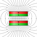  flat cylinder magnets with gap

• 
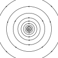  current in a wire
• 
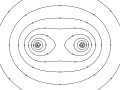  two parallel wires
• 
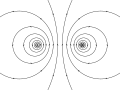  antiparallel wires
• 
  four antiparallel wires
• 
  six wires with alternating direction
• 
  eight wires with antiparallel direction
• 
  ring current
• 
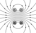  Helmholtz coil
• 
  anti-Helmholtz coil
• 
  Maxwell coil
• 
  Barker coil with three rings
• 
  Barker coil with four rings
• 
  Braunbek coil
• 
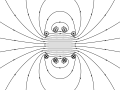  Fanselau coil
• 
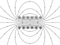  solenoid with finite windings
• 
  ideal solenoid
• 
  ideal solenoid
• 
  quadrupole solenoids
• 
  field of a helmholtz coil

• 
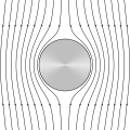  B-field around a conducting cylinder in a homogeneous field
• 
  B-field around a superconductor
• 
  E-field around a conducting cylinder in a homogeneous field
• 
  E-field around a conducting ball

• 
  positive charge
• 
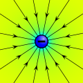  negative charge
• 
  E-field around two opposite charges
• 
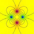  E-field around four charges on a square
• 
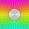  B-field around a conducting cylinder in a homogeneous field
• 
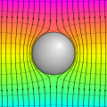  B-field around a conducting ball in a homogeneous field
• 
  E-field around a conducting cylinder in a homogeneous field
• 
  E-field around a conducting ball in a homogeneous field
• 
  E-field around oppositely charged balls
• 
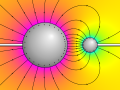  E-field around different oppositely charged balls
• 
  E-field around equally charged balls
• 
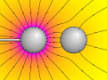  E-field around one charged and one neutral ball
• 
  E-field around infinite capacitor
• 
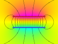  E-field around square capacitor
• 
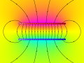  E-field around round capacitor
• 
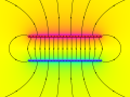  E-field around rod capacitor
• 
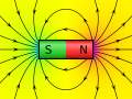  cylindrical bar magnet
• 
  flat cylinder magnet
• 
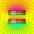  flat cylinder magnets with gap
• 
  spherical magnet

• 
  E-field around an infinite charged sheet at constant potential
• 
  E-field around an infinite uniformly charged sheet
• 
  E-field around an infinite charged wire
• 
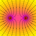  E-field around two equally charged infinite wires
• 
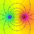  E-field around two oppositely charged infinite wires
• 
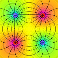  E-field around four alternatingly charged wires
• 
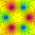  E-field around six alternatingly charged wires
• 
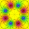  E-field around eight alternatingly charged wires
• 
  E-field around alternatingly charged wires

Improvements and bugs

VectorFieldPlot is some complicated piece of code. There may still be some bugs that wait for their chance to appear. If you should discover one or you are confronted with some strange behaviour, the best way is to use the discussions page. Avoid making modifications to the source code at this page directly, since those may get overwritten. If you should have ideas, improvements or patches, post it at the discussions page or create your own clone of VectorFieldPlot according to the licence terms.

Future developments

VectorFieldPlot is extensible in many imaginable ways. The most likely extensions that may come up in the forseeable future, are:

• creation of animations
• inclusion of metal surfaces

Licence

VectorFieldPlot is licensed under the terms of the GNU General Public License (https://www.gnu.org/licenses/gpl.html). This makes it free software.