File:Savitzky-golay pic gaussien bruite.svg
Jump to navigation
Jump to search

Size of this PNG preview of this SVG file: 610 × 407 pixels. Other resolutions: 320 × 214 pixels | 640 × 427 pixels | 1,024 × 683 pixels | 1,280 × 854 pixels | 2,560 × 1,708 pixels.
Original file (SVG file, nominally 610 × 407 pixels, file size: 43 KB)
Captions
Captions
Add a one-line explanation of what this file represents
Summary[edit]
| Description |
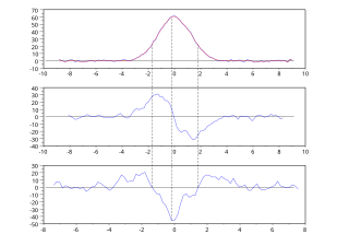
English: Savitzky-Golay algorithm (3rd degree polynomial, 9 points) applied on a gaussian peak with random noise: smoothing (top), first derivation (middle), second derivation (bottom).
The dashed lines highlight the zeros of the second dérivative (inflection points of the peak) and its minimum (top of the peak). Created with Scilab, processed with Inkscape.Français : Application de l'algorithme de Savitzky-Golay sur un pic gaussien bruité (polynôme de degré 3, 9 points) : lissage (haut), dérivée (milieu), dérivée seconde (bas).
Les traits pointillés mettent en évidence l'annulation de la dérivée seconde (points d'inflexion du pic) et son minimum (sommet du pic). Créé avec Scilab, retravaillé avec Inkscape. |
| Date | |
| Source | Own work |
| Author | Christophe Dang Ngoc Chan |
| SVG development |  English: English version by default.
Français : Version française, si les préférences de votre compte sont réglées (voir Special:Preferences). This vector image was created with Scilab. This file uses embedded text. |
| Source code | (1) File generateur_pic_bruit.sce : generates a set of data and save it in the file noisy_gaussian_peak.txt.
SciLab code// **********
// Constants and initialisation
// **********
clear;
chdir("mypath/");
// parameters of the noisy curve
paramgauss(1) = 60; // height of the gaussian curve
paramgauss(2) = 3; // "width" of the gaussian curve
var=0.01; // variance of the noise normal law
nbpts = 100 // nombre of points
halfwidth = 3*paramgauss(2) // range for x
step = 2*halfwidth/nbpts;
// **********
// Fonctions
// **********
// gaussian peak
function [y] = gauss(A, x)
// A(1) : height of the peak
// A(2) : "width" of the peak
y = A(1)*exp(-x.^2/A(2));
endfunction
// **********
// Main program
// **********
// Generation of data
for i=1:nbpts
x = step*i - halfwidth;
X(i) = x;
Y(i) = gauss([paramgauss], x) + rand(var, "normal");
end
// Saving the data
write ("noisy_gaussian_peak.txt", [X, Y])
(2) File savitzkygolay.sce : processes the data.
Data// **********
// Constants and initialisation
// **********
clear;
clf;
chdir("mypath/")
// smoothing parameters :
width = 9; // width of the sliding window (number of pts)
poldeg = 3; // degree of the polynomial
// **********
// Functions
// **********
// Convolution coefficients
function [a]=convolcoefs(m, d)
// m : width of the window (number of pts)
// d : degree of the polynomial
l = (m-1)/2; // half-width of the window
z = (-l:l)'; // standardised abscissa
J = ones(m,d+1);
for i = 2:d+1
J(:,i) = z.^(i-1); // jacobian matrix
end
A = (J'*J)^(-1)*J';
a = A(1:3,:);
endfunction
// smoothing, determination of the first and second derivatives
function [y, yprime, ysecond] = savitzkygolay(X, Y, width, deg)
// X, Y: collection of data
// width: width of the window (number of pts)
// deg: degree of the polynomial
n = size(X, "*");
l = floor(width/2);
step = (X($)-X(1))/(n - 1);
y = Y;
yprime=zeros(Y);
ysecond=yprime;
a = convolcoefs(width, deg);
a(2,:) = 1/step*a(2,:);
a(3,:) = 2/step^2*a(2,:);
for i = 1:width
Ymat(i, :) = Y(i: n-width+i)';
end
solution = a*Ymat;
y = solution(1, :)';
yprime = solution(2, :)';
ysecond = solution(3, :)';
endfunction
// **********
// Main program
// **********
// data reading
data = read("noisy_gaussian_peak.txt", -1, 2)
Xinit = data(:,1);
Yinit = data(:,2);
//subplot(3,1,1)
//plot(Xdef, Ydef, "b")
// Data processing
[Ysmooth, Yprime, Ysecond] = savitzkygolay(Xinit, Yinit, width, poldeg);
// Display
offset = floor(width/2);
nbpts = size(Xinit, "*");
X1 = Xinit((offset+1):(nbpts-offset)); // removal of non-smotthed points
subplot(3,1,1)
plot(Xinit, Yinit, "b")
plot(X1, Ysmooth, "r")
subplot(3,1,2)
plot(X1, Yprime, "b")
subplot(3,1,3)
plot(X1, Ysecond, "b")
(3) When the sampling step is not constant, i.e. xi - xi - 1 varies, then it is possible to determine the polynomial by multi-linear regression. Text// **********
// Constants and initialisation
// **********
clear;
clf;
chdir("mypath\")
// smoothing parameters
width = 9; // width of the sliding window (number of pts)
// **********
// Functions
// **********
// 3rd degree polynomial
function [y]=poldegthree(A, x)
// Horner method
y = ((A(1).*x + A(2)).*x + A(3)).*x + A(4);
endfunction
// regression with the 3rd degree polynomial
function [A]=regression(X, Y)
// X, Y: column vectors of "width" values ;
// determines the polynomial of degree 3
// a*x^2 + b*x^2 + c*x + d
// by regression on (X, Y)
XX = [X.^3; X.^2; X];
[a, b, sigma] = reglin(XX, Y);
A = [a, b];
endfunction
// smoothing, determination of the first and second derivatives
function [y, yprime, ysecond] = savitzkygolay(X, Y, larg)
// X, Y: collection of data
n = size(X, "*");
l = floor(larg/2); // halfwidth
y=Y;
yprime=zeros(Y);
ysecond=yprime;
for i=(l+1):(n-l)
intervX = X((i-l):(i+l),1);
intervY = Y((i-l):(i+l),1);
Aopt = regression(intervX', intervY');
x = X(i);
y(i) = poldegthree(Aopt,x);
// Yfoo=poldegthree(Aopt,intervX);
// subplot(3,1,1) ; plot(intervX, Yfoo, "r")
yprime(i) = (3*Aopt(1)*x + 2*Aopt(2))*x + Aopt(3); // Horner
ysecond(i) = 6*Aopt(1)*x + 2*Aopt(2);
end
endfunction
// **********
// Main program
// **********
// data reading
data = read("noisy_gaussian_peak.txt", -1, 2)
Xinit = data(:,1);
Yinit = data(:,2);
//subplot(3,1,1)
//plot(Xdef, Ydef, "b")
// Data processing
[Ysmooth, Yprime, Ysecond] = savitzkygolay(Xinit, Yinit, width);
// Display
offset = floor(width/2);
nbpts = size(Xinit, "*");
vector1 = (offset+1):(nbpts-offset); // suppresion des points non-lissés
X1 = Xinit(vector1);
Y0 = Yliss(vector1)
Y1 = Yprime(vector1);
Y2 = Ysecond(vector1);
subplot(3,1,1)
plot(Xinit, Yinit, "b")
plot(X1, Y0, "r")
subplot(3,1,2)
plot(X1, Y1, "b")
subplot(3,1,3)
plot(X1, Y2, "b")
|
Licensing[edit]
I, the copyright holder of this work, hereby publish it under the following licenses:

|
Permission is granted to copy, distribute and/or modify this document under the terms of the GNU Free Documentation License, Version 1.2 or any later version published by the Free Software Foundation; with no Invariant Sections, no Front-Cover Texts, and no Back-Cover Texts. A copy of the license is included in the section entitled GNU Free Documentation License. |
This file is licensed under the Creative Commons Attribution-Share Alike 3.0 Unported, 2.5 Generic, 2.0 Generic and 1.0 Generic license.
- You are free:
- to share – to copy, distribute and transmit the work
- to remix – to adapt the work
- Under the following conditions:
- attribution – You must give appropriate credit, provide a link to the license, and indicate if changes were made. You may do so in any reasonable manner, but not in any way that suggests the licensor endorses you or your use.
- share alike – If you remix, transform, or build upon the material, you must distribute your contributions under the same or compatible license as the original.
You may select the license of your choice.
File history
Click on a date/time to view the file as it appeared at that time.
| Date/Time | Thumbnail | Dimensions | User | Comment | |
|---|---|---|---|---|---|
| current | 13:07, 9 November 2012 | | 610 × 407 (43 KB) | Cdang (talk | contribs) | dashed line to highlight the inimum of the second derivative |
| 10:50, 9 November 2012 |  | 610 × 407 (43 KB) | Cdang (talk | contribs) | {{Information | description = {{en|1=Savitzky-Golay algorithm (3<sup>rd</sup> degree polynomial, 9 points) applied on a gaussian peak with random noise: smoothing (top), first derivation (middle), second derivation (bottom). Created with Scilab, proce... |
You cannot overwrite this file.
File usage on Commons
There are no pages that use this file.
File usage on other wikis
The following other wikis use this file:
- Usage on es.wikipedia.org
- Usage on fr.wikipedia.org
- Usage on fr.wikibooks.org
- Usage on nl.wikipedia.org