File:Solar AM0 spectrum with visible spectrum background (no).png
Jump to navigation
Jump to search

Size of this preview: 800 × 494 pixels. Other resolutions: 320 × 198 pixels | 640 × 395 pixels | 1,024 × 632 pixels | 1,280 × 790 pixels | 1,882 × 1,162 pixels.
Original file (1,882 × 1,162 pixels, file size: 182 KB, MIME type: image/png)
Captions
Captions
Add a one-line explanation of what this file represents
Summary
[edit].png&action=edit§ion=1)
| Description |
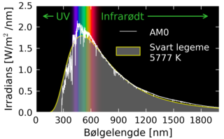
English: Solar AM0 (Air Mass Zero) spectrum (Chris A. Gueymard 2002) as included in SMARTS 2.95, together with a blackbody spectrum for 5777 kelvin and solid angle 2.16e-5*π steradian for the source (the solar disk). The visible region of the electromagnetic spectrum is shown using the CIE visible spectrum as implemented in ColorPy by Mark Kness (2008). Figure with Norwegian Bokmål labels. |
| Date | |
| Source | Own work, created using Matplotlib |
| Author | Danmichaelo |
| Other versions | Version with English labels |
.png)
Source
|
|---|
#encoding=utf8

import matplotlib
from matplotlib import rc
from matplotlib import pyplot as plt
import numpy as np

rc('lines', linewidth=0.5)
rc('font', family='sans-serif', size=10)
rc('axes', labelsize=10)
rc('xtick', labelsize=9)
rc('ytick', labelsize=9)

golden_mean = (np.sqrt(5)-1.0)/2.0
inches_per_cm = 1.0/2.54
fig_width = 8 * inches_per_cm
fig_height = golden_mean * fig_width
fig = plt.figure(figsize = [fig_width, fig_height])

from colorpy import ciexyz, colormodels

Fs = 2.16e-5 * np.pi;   # Geometrical factor of sun as viewed from Earth
h = 6.63e-34;           # Boltzmann const. [Js]
c = 3.e8;               # speed of light [m/s]
q = 1.602e-19;          # electron charge [C]

def blackbody(wvlgth, temp):
    # per nanometer 1e-9:
    fac = (2 * Fs * h * c**2) / ((wvlgth * 1.e-9)**5)
    return fac / (np.exp(1240./(wvlgth*8.62e-5*temp)) - 1) * 1.e-9

def draw_vis_spec(ax, ymax):
    spectrum = ciexyz.empty_spectrum()[:,0]
    (num_wl,) = spectrum.shape
    rgb_colors = np.empty((num_wl, 3))
    for i in xrange (0, num_wl):
        xyz = ciexyz.xyz_from_wavelength(spectrum[i])
        rgb = colormodels.rgb_from_xyz(xyz)
        rgb_colors [i] = rgb
    rgb_colors /= np.max(rgb_colors) # scale to make brightest rgb value = 1.0

    num_points = len(spectrum)
    for i in xrange (0, num_points-1):
        x0 = spectrum[i]
        x1 = spectrum[i+1]
        y0 = 0.0
        y1 = ymax
        poly_x = [x0, x1, x1, x0]
        poly_y = [y0, y0, y1, y1]
        color_string = colormodels.irgb_string_from_rgb(rgb_colors [i])
        ax.fill(poly_x, poly_y, color_string, edgecolor=color_string)

ax = fig.add_subplot(111)

frame = ax.get_frame()
frame.set_facecolor('black')
xmax = 2000
ymax = 2.5

# Visible spectrum:

draw_vis_spec(ax, ymax)

# Blackbody:

temp = 5777
x = np.arange(100, 2000)
y = blackbody(x, temp)
y[-1] = 0.
ax.fill(x, y, '0.5', alpha = 0.7, linewidth = 0.9, edgecolor='yellow', label = 'Svart legeme\n%d K' % temp)

# AM0 spectrum:

d = np.loadtxt('smarts295.ext.txt', skiprows = 1)
x = d[:,0]
y = d[:,1]
y[0] = 0.
y[-1] = 0.
ax.plot(x, y, color='white', linewidth=0.5, label = 'AM0')
ax.set_xlim(0, xmax)
ax.set_xticks(np.arange(0, 1999, 300))
ax.set_ylim(0, ymax)

# Tweak, tweak and annotate:

texty = 2.25
ax.annotate('UV', xy = (50,texty), xytext = (230,texty), xycoords = 'data',
        horizontalalignment='left', verticalalignment='center', color='#33bb33',
        arrowprops = dict(arrowstyle='->', color='#33bb33'))
#ax.annotate('Synlig', xy=(400,texty), xycoords='data',
#        horizontalalignment='left', verticalalignment='center', color='white')
ax.annotate(u'Infrarødt', xytext = (720,texty), xy = (1900,texty), xycoords = 'data',
        horizontalalignment='left', verticalalignment='center', color='#33bb33',
        arrowprops = dict(arrowstyle='->',color='#33bb33'))

leg = ax.legend(loc='upper right', frameon=False, bbox_to_anchor = (1.0, 0.90) )
txts = leg.get_texts()
for txt in txts:
    txt.set_color('white')
    txt.set_fontsize(9)

ax.tick_params(color='white', labelcolor='black')
for spine in ax.spines.values():
    spine.set_edgecolor('white')
    spine.set_linewidth(1.4)

fig.subplots_adjust(left=0.16, bottom = 0.19, right=0.98, top=0.96)

ax.set_xlabel(u'Bølgelengde [nm]')
ax.set_ylabel(u'Irradians [W/m$^2$/nm]')
fig.savefig('Solar AM0 spectrum with visible spectrum background (no).png',dpi=600)
|
Licensing
[edit].png&action=edit§ion=2)
| I, the copyright holder of this work, release this work into the public domain. This applies worldwide. In some countries this may not be legally possible; if so: I grant anyone the right to use this work for any purpose, without any conditions, unless such conditions are required by law. |
File history
Click on a date/time to view the file as it appeared at that time.
| Date/Time | Thumbnail | Dimensions | User | Comment | |
|---|---|---|---|---|---|
| current | 20:16, 16 May 2012 | | 1,882 × 1,162 (182 KB) | Danmichaelo (talk | contribs) | slightly thicker line |
| 19:30, 16 May 2012 |  | 1,882 × 1,162 (181 KB) | Danmichaelo (talk | contribs) | tweaks to make the figure more readable | |
| 19:12, 16 May 2012 |  | 1,882 × 1,162 (171 KB) | Danmichaelo (talk | contribs) |
You cannot overwrite this file.
File usage on Commons
There are no pages that use this file.
.png&oldid=840021303)