File:AdaptiveBeamForming.png
Jump to navigation
Jump to search

Size of this preview: 800 × 405 pixels. Other resolutions: 320 × 162 pixels | 640 × 324 pixels | 1,291 × 653 pixels.
Original file (1,291 × 653 pixels, file size: 78 KB, MIME type: image/png)
Captions
Captions
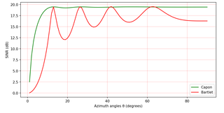
Signal-to-Noise-plus-Interference performance of the Capon's and Bartlett's beamforming methods.
Summary[edit]
| Description |
English: An example of Adaptive Beamforming (source code).
Русский: Пример адаптивного диаграммообразования (исходный код). |
| Date | |
| Source | Own work |
| Author | Kirlf |
| PNG development | This plot was created with Matplotlib. |
| Source code | Python code"""
Developed by Vladimir Fadeev
(https://github.com/kirlf)
Kazan, 2017 / 2020
Python 3.7
"""
import numpy as np
import matplotlib.pyplot as plt
"""
Received signal model:
X = A*S + N
where
A = [a(theta_1) a(theta_2) ... a(theta_d)]
is the matrix of steering vectors
(dimension is M x d,
M is the number of sensors,
d is the number of signal sources),
A steering vector represents the set of phase delays
a plane wave experiences, evaluated at a set of array elements (antennas).
The phases are specified with respect to an arbitrary origin.
theta is Direction of Arrival (DoA),
S = 1/sqrt(2) * (X + iY)
is the transmit (modulation) symbols matrix
(dimension is d x T,
T is the number of snapshots)
(X + iY) is the complex values of the signal envelope,
N = sqrt(N0/2)*(G1 + jG2)
is additive noise matrix (AWGN)
(dimension is M x T),
N0 is the noise spectral density,
G1 and G2 are the random Gussian distributed values.
"""
M = 9 # number of antenna elements (sensors)
""" Correlation matrix of the information symbols:
Rss = S*S^H = I_d (try with QPSK, for example) """
Rss = np.eye((2))
""" Correlation matrix of additive noise:
Rnn = N*N^H = sigma_N^2 * I_M),
where sigma_N^2 is the noise variance (power) """
Rnn = 0.1*np.eye((M)) #
""" Let us consider 2 sources of the signals """
theta_1 = 0*(np.pi/180)
theta_2 = 50*(np.pi/180)
""" Spatial frequency (some equivalent of a DoA):
mu = (2*pi / lambda ) * delta * sin(theta)
where
delta is the antenna spacing
(distance between antenna elements), and
lambda is the electromagnetic wave length.
Let us (delta = lambda / 2) then:
"""
mu_1 = np.pi*np.sin(theta_1)
mu_2 = np.pi*np.sin(theta_2)
""" Steering vectors """
a_1 = np.exp(1j*mu_1*np.arange(M))
a_2 = np.exp(1j*mu_2*np.arange(M))
A = (np.array([a_1, a_2])).T
"""
Correlation matrix of the received signals
R_xx = X*X^H = A*R_ss*A^H + R_nn
"""
R = A @ Rss @ np.conj(A).T + Rnn
""" Let us theta_1 is the signal, and theta_2 is the interferer """
g = np.array([1, 0]) # the first DoA is "switched on", the second DoA is "switched off".
def calc_w_capon(A_i):
""" Capon's method (MVDR)
w_Capon = R^(-1) * A * (A^H * R^(-1) * A)^(-1) * g """
w = (np.linalg.inv(R) @ A_i @
np.linalg.inv( np.conj(A_i).T @ np.linalg.inv(R) @ A_i ) @ g).T
return w
def calc_power(w, a):
""" P(theta) = abs(w_(opt)^H * a(theta))^2 """
P = (np.abs( (np.conj(w).T @ a) )**2).item()
return P
""" Bartlett's method (сonventional beamforming)
w_Bart = a_1 / M """
w_bart = (a_1 / M).reshape((M,1))
""" Simulation loop.
Main idea:
1) We have the Rxx matrix from the receiver.
2) We know the DoA of the information signal and
DoA of the interference (e.g., based on frequency estimation methods)
3) We should calculate optimal weight vector which will suppress interference.
4) This should make SINR (Signal to Interference + Noise Ratio) better.
5) Interference DoA can changes, but estimated Rxx should be the same!
"""
sinr_thetas = np.arange(1, 91)*(np.pi/180) # degrees (from 1 to 90) -> radians
SINR_Capon = np.empty(len(sinr_thetas), dtype = complex)
SINR_Bart = np.empty(len(sinr_thetas), dtype = complex)
for idx, theta_i in enumerate(sinr_thetas):
""" Let's try to simulate changing of the interference picture!
For this redefine DoA of intereference. """
mu_2 = np.pi*np.sin(theta_i)
a_2 = np.exp(1j*mu_2*np.arange(M))
A_sinr = (np.array([a_1, a_2])).T
""" Capon's (MVDR) method: """
w_capon = calc_w_capon(A_sinr)
signal_capon = calc_power(w_capon, a_1)
interf_capon = calc_power(w_capon, a_2)
""" P_noise = w^H * Rnn * w """
noise_capon = (np.conj(w_capon).T @ Rnn @ w_capon).item()
""" SINR - Signal to Interference + Noise Ratio """
SINR_Capon[idx] = signal_capon / (interf_capon + noise_capon)
""" Bartlett's method
(uses the same weight vector for every cases - not adaptive): """
signal_bart = calc_power(w_bart, a_1)
interf_bart = calc_power(w_bart, a_2)
noise_bart = (np.conj(w_bart).T @ Rnn @ w_bart).item()
SINR_Bart[idx] = signal_bart / (interf_bart + noise_bart)
"""
Capon's method is more stable,
Bartlett's method cannot well mitigate changed interference.
"""
plt.subplots(figsize=(10, 5), dpi=150)
plt.plot(sinr_thetas*(180/np.pi), 10*np.log10(np.real(SINR_Capon)), color='green', label='Capon')
plt.plot(sinr_thetas*(180/np.pi), 10*np.log10(np.real(SINR_Bart)), color='red', label='Bartlett')
plt.grid(color='r', linestyle='-', linewidth=0.2)
plt.xlabel('Azimuth angles θ (degrees)')
plt.ylabel('SINR (dB)')
plt.legend()
plt.show()
""" References
1. Haykin, Simon, and KJ Ray Liu.
Handbook on array processing and sensor networks.
Vol. 63. John Wiley & Sons, 2010. pp. 102-107
2. Haykin, Simon S.
Adaptive filter theory.
Pearson Education India, 2008. pp. 422-427
3. Richmond, Christ D.
"Capon algorithm mean-squared error threshold
SNR prediction and probability of resolution." IEEE
"""
|
Licensing[edit]
I, the copyright holder of this work, hereby publish it under the following license:
This file is licensed under the Creative Commons Attribution-Share Alike 4.0 International license.
- You are free:
- to share – to copy, distribute and transmit the work
- to remix – to adapt the work
- Under the following conditions:
- attribution – You must give appropriate credit, provide a link to the license, and indicate if changes were made. You may do so in any reasonable manner, but not in any way that suggests the licensor endorses you or your use.
- share alike – If you remix, transform, or build upon the material, you must distribute your contributions under the same or compatible license as the original.
File history
Click on a date/time to view the file as it appeared at that time.
| Date/Time | Thumbnail | Dimensions | User | Comment | |
|---|---|---|---|---|---|
| current | 05:37, 18 February 2019 | | 1,291 × 653 (78 KB) | Kirlf (talk | contribs) | User created page with UploadWizard |
You cannot overwrite this file.
File usage on Commons
There are no pages that use this file.
File usage on other wikis
The following other wikis use this file:
- Usage on ru.wikipedia.org