File:VFPt ringmagnet2 potential+contour.svg

From Wikimedia Commons, the free media repository
Jump to navigation Jump to search

Original file(SVG file, nominally 600 × 600 pixels, file size: 199 KB)

Captions

Captions

Add a one-line explanation of what this file represents

Summary

[edit]
Description
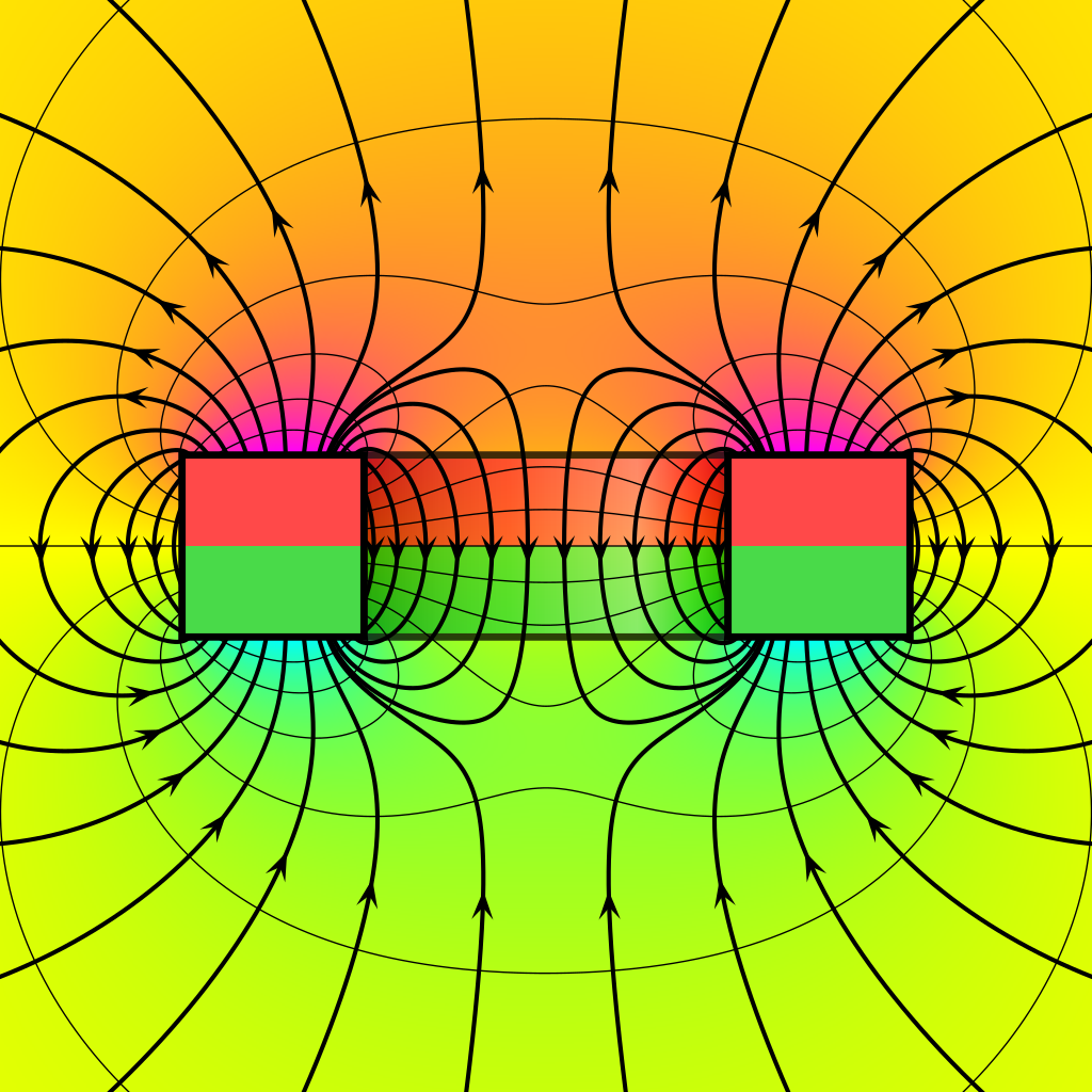
English: Drawing of a cylindrical ringmagnet with precisely computed magnetic field lines. The magnet consists of a flat cylinder of R/L=2 with a cylindrical hole of radius r/R=1/2 and is homogeneously magnetized along the cylinder axis. The north-half of the magnet is painted red, whereas the south-half is green. The precise field distribution is obtained by numerical integration. The shape of the field lines is traced with a Runge-Kutta algorithm. The density of field lines corresponds roughly to the field strength, however due to 3D variations of the field, this cannot exactly be fulfilled. The magnetic scalar potential 𝜓 is shown in the background from positive (fuchsia) through zero (yellow) to negative (aqua) together with uniformely spaced equipotential lines. Note that the field lines follow the gradient of the scalar potential.
Date
Source Own work
Author Geek3
SVG development
InfoField
 
The SVG code is valid.
 
This plot was created with VectorFieldPlot.
Source code
InfoField

Python code

Python VectorFieldPlot code
# paste this code at the end of VectorFieldPlot 3.3
# https://commons.wikimedia.org/wiki/User:Geek3/VectorFieldPlot
doc = FieldplotDocument('VFPt_ringmagnet2_potential+contour',
    commons=True, width=600, height=600)

r0 = 1.0
r1 = 2.0
h = 0.5
Bfield = Field([ ['coil', {'x':0, 'y':0, 'phi':pi/2, 'R':r1, 'Lhalf':h, 'I':1}],
         ['coil', {'x':0, 'y':0, 'phi':pi/2, 'R':r0, 'Lhalf':h, 'I':-1}] ])
Hfield = Field([ ['charged_disc', {'x0':-r1, 'y0':-h, 'x1':r1, 'y1':-h, 'Q':-pi*r1**2/(2*h)}],
    ['charged_disc', {'x0':-r0, 'y0':-h, 'x1':r0, 'y1':-h, 'Q':pi*r0**2/(2*h)}],
    ['charged_disc', {'x0':-r1, 'y0':h, 'x1':r1, 'y1':h, 'Q':pi*r1**2/(2*h)}],
    ['charged_disc', {'x0':-r0, 'y0':h, 'x1':r0, 'y1':h, 'Q':-pi*r0**2/(2*h)}] ])

U1 = Hfield.V([0, 2])

n_out = 24
for i in range(n_out):
    s = (i + 0.5) / n_out * 2. - 1.
    line = FieldLine(Bfield, [copysign(r1 + h * (1. / s**2 - 1.), s), 0.],
        directions='both', maxr=1e3)
    doc.draw_line(line, linewidth=2.4, arrows_style={'scale':1.1,
        'potential':Hfield.V, 'at_potentials':[-U1, 0, U1],
        'condition_func':lambda xy: fabs(xy[1]) > 0.7 or
            (fabs(xy[0]) > r1 and fabs(xy[1]) < 1e-4)})

n_in = 12
for i in range(n_in):
    a = (i + 0.5) / n_in * 2. - 1.
    line = FieldLine(Bfield, [r0 * (1.2*a - 0.2*a**3), 0.],
        directions='both')
    doc.draw_line(line, linewidth=2.4, arrows_style={'scale':1.1,
        'potential':lambda xy: xy[1], 'at_potentials':[0],
        'condition_func':lambda xy: fabs(xy[0]) < r0})

U0 = Hfield.V([0.5 * (r0 + r1), h])
doc.draw_scalar_field(func=Hfield.V, cmap=doc.cmap_AqYlFs, vmin=-U0, vmax=U0)
doc.draw_contours(func=Hfield.V, levels=sc.linspace(-U0, U0, 15)[1:-1])

# draw the magnet manually
colors = ['#00cc00', '#ff0000']
defs = doc.draw_object('defs', {})
grad = doc.draw_object('linearGradient', {'id':'grad',
    'x1':str(r0), 'x2':str(-r0), 'y1':'0', 'y2':'0',
    'gradientUnits':'userSpaceOnUse'}, group=defs)
for col, of, opa in [['#000000', '0', '0.4'], ['#000000', '0.03', '0.125'],
    ['#ffffff', '0.1', '0.125'], ['#ffffff', '0.25', '0.5'],
    ['#ffffff', '0.6', '0.2'], ['#000000', '1', '0.3'], ['#000000', '1', '0.5']]:
    stop = doc.draw_object('stop', {'stop-color':col, 'offset':of,
        'stop-opacity':opa}, group=grad)
mag = doc.draw_object('g', {'id':'magnet', 'opacity':0.7}, bg=True)
for i in [0, 1]:
    rect = doc.draw_object('rect', group=mag)
    for attr, val in [['x', -r0], ['y', [-h, 0][i]],
        ['width', 2*r0], ['height', [2*h, h][i]],
        ['style', 'fill:{0}; stroke:none'.format(colors[i])]]:
        rect.set(attr, str(val))
rect = doc.draw_object('rect', group=mag)
for attr, val in [['x', -r0], ['y', -h],
    ['width', 2 * r0], ['height', 2 * h],
    ['style', 'fill:url(#grad); stroke-width:0.04; stroke-linejoin:miter; stroke:#000000']]:
    rect.set(attr, str(val))

for x0 in [-r1, r0]:
    mag = doc.draw_object('g')
    for i in [0, 1]:
        rect = doc.draw_object('rect', group=mag)
        for attr, val in [['x', x0], ['y', [-h, 0][i]],
            ['width', r1 - r0], ['height', [2*h, h][i]],
            ['style', 'fill:{0}; stroke:none'.format(
            ['#49da49', '#ff4949'][i])]]:
            rect.set(attr, str(val))
    rect = doc.draw_object('rect', group=mag)
    for attr, val in [['x', x0], ['y', -h],
        ['width', r1 - r0], ['height', 2 * h],
        ['style', 'fill:none; stroke-width:0.04; stroke-linejoin:miter; stroke:#000000']]:
        rect.set(attr, str(val))

doc.write()

Licensing

[edit]
I, the copyright holder of this work, hereby publish it under the following license:
w:en:Creative Commons
attribution share alike
This file is licensed under the Creative Commons Attribution-Share Alike 4.0 International license.
You are free:
  • to share – to copy, distribute and transmit the work
  • to remix – to adapt the work
Under the following conditions:
  • attribution – You must give appropriate credit, provide a link to the license, and indicate if changes were made. You may do so in any reasonable manner, but not in any way that suggests the licensor endorses you or your use.
  • share alike – If you remix, transform, or build upon the material, you must distribute your contributions under the same or compatible license as the original.

File history

Click on a date/time to view the file as it appeared at that time.

Date/TimeThumbnailDimensionsUserComment
current15:42, 16 December 2022Thumbnail for version as of 15:42, 16 December 2022600 × 600 (199 KB)Geek3 (talk | contribs)Uploaded own work with UploadWizard

There are no pages that use this file.

Metadata