File:VFPt metal balls positive transparent.svg
Jump to navigation
Jump to search

Size of this PNG preview of this SVG file: 800 × 600 pixels. Other resolutions: 320 × 240 pixels | 640 × 480 pixels | 1,024 × 768 pixels | 1,280 × 960 pixels | 2,560 × 1,920 pixels.
Original file (SVG file, nominally 800 × 600 pixels, file size: 49 KB)
Captions
Captions
Add a one-line explanation of what this file represents
Summary
[edit]| Description |
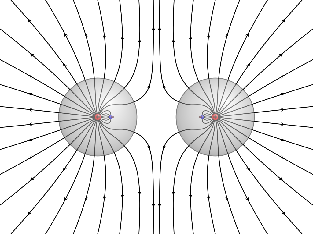
English: Electric field around two identical positively charged conducting spheres. The shape of the field lines is computed exactly, using the method of image charges with an infinite series of charges inside the two spheres, shown in red and blue. In reality, the field is created by a continuous charge distribution at the surface of each sphere and the field lines inside the sphere don't exist. Field lines are always orthogonal to the surface of each sphere. |
| Date | |
| Source | Own work |
| Author | Geek3 |
| Other versions |
|
| SVG development | |
| Source code | Python code# paste this code at the end of VectorFieldPlot 1.10
# https://commons.wikimedia.org/wiki/User:Geek3/VectorFieldPlot
u = 100.0
doc = FieldplotDocument('VFPt_metal_balls_positive_transparent',
commons=True, width=800, height=600, center=[400, 300], unit=u)
# define two spheres with position, radius and charge
s1 = {'p':sc.array([-1.5, 0.]), 'r':1.0, 'q':1.}
s2 = {'p':sc.array([1.5, 0.]), 'r':1.0, 'q':1.}
d = vabs(s2['p'] - s1['p'])
v12 = (s2['p'] - s1['p']) / d
# compute series of charges https://dx.doi.org/10.2174/1874183500902010032
charges = [[s1['p'][0], s1['p'][1], s1['q']], [s2['p'][0], s2['p'][1], s2['q']]]
r1 = r2 = 0.
q1, q2 = s1['q'], s2['q']
q0 = max(fabs(q1), fabs(q2))
for i in range(10):
q1, q2 = -s1['r'] * q2 / (d - r2), -s2['r'] * q1 / (d - r1),
r1, r2 = s1['r']**2 / (d - r2), s2['r']**2 / (d - r1)
p1, p2 = s1['p'] + r1 * v12, s2['p'] - r2 * v12
charges.append([p1[0], p1[1], q1])
charges.append([p2[0], p2[1], q2])
if max(fabs(q1), fabs(q2)) < 1e-3 * q0:
break
field = Field({'monopoles':charges})
# draw symbols
for c in charges:
doc.draw_charges(Field({'monopoles':[c]}), scale=0.6*sqrt(fabs(c[2])))
gradr = doc.draw_object('linearGradient', {'id':'rod_shade', 'x1':0, 'x2':0,
'y1':0, 'y2':1, 'gradientUnits':'objectBoundingBox'}, group=doc.defs)
for col, of in (('#666', 0), ('#ddd', 0.6), ('#fff', 0.7), ('#ccc', 0.75),
('#888', 1)):
doc.draw_object('stop', {'offset':of, 'stop-color':col}, group=gradr)
gradb = doc.draw_object('radialGradient', {'id':'metal_spot', 'cx':'0.53',
'cy':'0.54', 'r':'0.55', 'fx':'0.65', 'fy':'0.7',
'gradientUnits':'objectBoundingBox'}, group=doc.defs)
for col, of in (('#fff', 0), ('#e7e7e7', 0.15), ('#ddd', 0.25),
('#aaa', 0.7), ('#888', 0.9), ('#666', 1)):
doc.draw_object('stop', {'offset':of, 'stop-color':col}, group=gradb)
ball_charges = []
for ib in range(2):
ball = doc.draw_object('g', {'id':'metal_ball{:}'.format(ib+1),
'transform':'translate({:.3f},{:.3f})'.format(*([s1, s2][ib]['p'])),
'style':'fill:none; stroke:#000;stroke-linecap:square', 'opacity':0.5})
# draw metal balls
doc.draw_object('circle', {'cx':0, 'cy':0, 'r':[s1, s2][ib]['r'],
'style':'fill:url(#metal_spot); stroke-width:0.02'}, group=ball)
ball_charges.append(doc.draw_object('g',
{'style':'stroke-width:0.02'}, group=ball))
# find start positions of field lines
def startpath(t):
phi = 2. * pi * t
return (s1['p'] + 1.4 * sc.array([cos(phi), sin(phi)]))
def dstartpath(t):
return (startpath(t+1e-6) - startpath(t-1e-6)) / 2e-6
def FieldSum(t0, t1):
return ig.quad(lambda t:
sc.cross(field.F(startpath(t)), dstartpath(t)), t0, t1)[0]
Ftotal = FieldSum(0, 1)
def startpos(s):
t = op.brentq(lambda t: FieldSum(0, t) / Ftotal - s, 0, 1)
return startpath(t)
# draw the field lines
p0_list = []
nlines = 22
for i in range(nlines):
p0_list.append(startpos((0.5 + i) / nlines))
for i in range(nlines):
p0_list.append(startpos((0.5 + i) / nlines) * sc.array([-1, 1]))
for phi in sc.linspace(-0.8, 0.8, 6):
p0_list.append(s1['p'] + 0.02 * sc.array([cos(phi), sin(phi)]))
for phi in sc.linspace(-0.8, 0.8, 6):
p0_list.append(s2['p'] + 0.02 * sc.array([-cos(phi), sin(phi)]))
for ip, p0 in enumerate(p0_list):
line = FieldLine(field, p0, directions='both', maxr=5.)
arrow_d = 1.7
of = [0.5 + s1['r'] / arrow_d, 0.5, 0.5, 0.5 + s2['r'] / arrow_d]
ma = 1
if ip >= len(p0_list) - 12:
ma = 0
doc.draw_line(line, arrows_style={'dist':arrow_d, 'offsets':of,
'min_arrows':ma})
doc.write()
|


Licensing
[edit]
I, the copyright holder of this work, hereby publish it under the following license:
This file is licensed under the Creative Commons Attribution-Share Alike 4.0 International license.
- You are free:
- to share – to copy, distribute and transmit the work
- to remix – to adapt the work
- Under the following conditions:
- attribution – You must give appropriate credit, provide a link to the license, and indicate if changes were made. You may do so in any reasonable manner, but not in any way that suggests the licensor endorses you or your use.
- share alike – If you remix, transform, or build upon the material, you must distribute your contributions under the same or compatible license as the original.
File history
Click on a date/time to view the file as it appeared at that time.
| Date/Time | Thumbnail | Dimensions | User | Comment | |
|---|---|---|---|---|---|
| current | 20:05, 30 December 2018 | | 800 × 600 (49 KB) | Geek3 (talk | contribs) | User created page with UploadWizard |
You cannot overwrite this file.
File usage on Commons
The following 3 pages use this file: