File:Ocean planet distance vs temperature moist energy balance model 1 1 1 1.png

Original file (1,070 × 700 pixels, file size: 90 KB, MIME type: image/png)
Captions
Captions
Summary
[edit]
| Description |
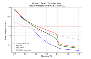
English: Ocean planet distance from Sun-like star effect to temperature - moist energy balance model. Assumed Sun-like star, ca 5778 K, and Earth-like but fully ocan covetred planet. Energy balance model that added moisture. |
| Date | |
| Source | Own work |
| Author | Merikanto |
Python3 climlab seasonal ebm code.
Note you must install climlab additional packages.
- must install additional packages along climlab
- pip install climlab
-
- and source pip install "pip install ." in source directory
- https://github.com/climlab/climlab-cam3-radiation
- https://github.com/climlab/climlab-emanuel-convection
- https://github.com/climlab/climlab-rrtmg
Python3 code
- 3
- orbital distance vs temperature of ocean planet
- seasonal climlab energy balance model
- python3/climlab code
- must install additional packages along climlab
- pip install climlab
-
- and source pip install "pip install ." in source directory
- https://github.com/climlab/climlab-cam3-radiation
- https://github.com/climlab/climlab-emanuel-convection
- https://github.com/climlab/climlab-rrtmg
- 17.11.2023 0000.0006a1
-
import math
import numpy as np
import matplotlib.pyplot as plt
from matplotlib import cm
from scipy.interpolate import griddata
import skimage
from skimage.transform import resize
import xarray as xr
import climlab
from climlab import constants as const
from climlab.process.diagnostic import DiagnosticProcess
from climlab.domain.field import Field, global_mean
from climlab.dynamics import MeridionalDiffusion
def plotmonths(Ts, lat):
	global title1
	lela=len(lat)
	print(np.shape(Ts))
	fig = plt.figure( figsize=(8,5) )
	ax = fig.add_subplot(111)
	clevels=10
	Tmin=-50
	Tmax=50
	plt.xticks(fontsize=15)
	plt.yticks(fontsize=15)
	cax = ax.contourf(np.arange(365)+0.5, lat, Ts,cmap=plt.cm.coolwarm,vmin=Tmin, vmax=Tmax, levels=256 )
	cc = ax.contour(np.arange(365)+0.5,  lat,  Ts, colors=['#00003f'],)
	ax.clabel(cc, cc.levels, colors=['#00005f'], inline=True, fmt='%3.1f',fontsize=15)
	#ax.set_tick_params(axis='both', which='minor', labelsize=15)
	ax.set_xlabel('Day', fontsize=15)
	ax.set_ylabel('Latitude', fontsize=15)
	#cbar = plt.colorbar(cax)
	#cbar.set_clim(-50.0, 50.0)
	ax.set_title('Zonal mean surface temperatures (degC)', fontsize=16)
	return(0)
def plotmonths2(model, Ts, lat):
	global title1
	#num_steps_per_year=360
	Tmin=np.min(Ts)
	Tmax=np.max(Ts)
	fig = plt.figure(figsize=(5,5))
	ax = fig.add_subplot(111)
	factor = 365. / num_steps_per_year
	#cmap1=plt.cm.seismic
	#cmap1=plt.cm.turbo
	cmap1=plt.cm.coolwarm
	#cmap1=plt.cm.winter
	#cmap1=plt.cm.cool_r
	#cmap1=plt.cm.cool
	#cmap1=cmap1.reversed()
	#levels1=[-80,-70,-60,-50,-40,-30]
	levels2=[-250,-200,-150,-120,-100,-90,-80,-70,-60,-50,-45,-40,-35,-30,-25,-20,-15,-10,-5,0,5,10,15,20,25,30,35,40,45,50,55,60,65,80,100,120,140,160,180,200,300,500]
	Tminv=-150
	Tmaxv=150
	#cax = ax.contourf(factor * np.arange(num_steps_per_year),
	#              ebm.lat, Tyear[:,:],
	#              cmap=cmap1, vmin=Tminv, vmax=Tmaxv, antialiased=False, levels=256)
	ax.imshow(Ts[:,:],origin="lower", extent=[0,360,-90,90],cmap=cmap1, vmin=Tminv, vmax=Tmaxv, interpolation="bicubic")
	cs1 = ax.contour(factor * np.arange(num_steps_per_year),model.lat, Ts[:,:], alpha=0.5,   origin="lower", extent=[0,360,-90,90],colors='#00005f', vmin=Tminv, vmax=Tmaxv, levels=levels2)
	ax.clabel(cs1, cs1.levels, inline=True, fontsize=14)
	#cbar1 = plt.colorbar(cax)
	ax.set_title(title1, fontsize=12)
	fig.suptitle(title0, fontsize=22)
	##ax_set_suptitle(title0, fontsize=18)
	ax.tick_params(axis='x', labelsize=12)
	ax.tick_params(axis='y', labelsize=12)
	ax.set_xlabel('Days of year', fontsize=13)
	ax.set_ylabel('Latitude', fontsize=13)
	#plt.tight_layout()
	plt.savefig('1000dpi.svg', dpi=1000)
	return(0)
class tanalbedo(DiagnosticProcess):
   def __init__(self, **kwargs):
       super(tanalbedo, self).__init__(**kwargs)
       self.add_diagnostic('albedo')
       Ts = self.state['Ts']
       self._compute_fixed()
   def _compute_fixed(self):
       Ts = self.state['Ts']
       try:
           lon, lat = np.meshgrid(self.lon, self.lat)
       except:
           lat = self.lat
       phi = lat
       try:
           albedo=np.zeros(len(phi));
           albedo=0.42-0.20*np.tanh(0.052*(Ts-3))
       except:
           albedo = np.zeros_like(phi)
       dom = next(iter(self.domains.values()))
       self.albedo = Field(albedo, domain=dom)
   def _compute(self):
       self._compute_fixed()
return {}
def model_ebm_00(Sk,ecc, long_peri, obliquity,albedo0,co20,waterdepth,cloudiness):
	num_years=30
	num_lev=4
	num_lat=36
	num_steps_per_year=72
	plotvar=0 ## 1,2,3 lot temp, ice, mean albedo
	#waterdepth=70
	S1=1361.5*Sk
	co2=co20
	#print(S1)
	diffu1=0.3 # meridional diffusivity in m**2/s
	#diffu1=1.0 # meridional diffusivity in m**2/s
	#diffu1=0.01
	#albedo0=0.28
	#orbit={'ecc': 0.0167643, 'long_peri': 280.32687, 'obliquity': 23.459277, 'S0':S1}
	orbit={'ecc': ecc, 'long_peri': long_peri, 'obliquity': obliquity, 'S0':S1}
	# creating EBM model
	#ebm= climlab.EBM(CO2=co2,orbit={'ecc': 0.0167643, 'long_peri': 280.32687, 'obliquity': 23.459277, 'S0':S1})
	#ebm0= climlab.EBM_seasonal(water_depth=10.0, a0=0.3, num_lat=90, lum_lon=None, num_lev=10,num_lon=None
	#, orbit=orbit)
	ebm0= climlab.EBM_seasonal(water_depth=waterdepth, a0=albedo0, num_lat=num_lat, lum_lon=None, num_lev=num_lev,num_lon=None)
	ebm=climlab.process_like(ebm0)
	#ebm.step_forward()
	#print(ebm.diagnostics)
	#quit(-1)
	surface = ebm.domains['Ts']
	# define new insolation and SW process
	ebm.remove_subprocess('insolation')
	insolation = climlab.radiation.DailyInsolation(domains=surface, orb = orbit, **ebm.param)
	insolation.S0=S1
	##sun = climlab.radiation.DailyInsolation(domains=model.Ts.domain)
	ebm.add_subprocess('insolation', insolation)
	#ebm.step_forward()
	#print(insolation.diagnostics)
	#print (insolation.insolation)
	#print (np.max(insolation.insolation))
	##print(insolation.S0)
	#quit(-1)
	#Tf=-10
	Tf=-10
	alb = climlab.surface.albedo.StepFunctionAlbedo(state=ebm.state, Tf=Tf, **ebm.param)
	#alb = climlab.surface.albedo.StepFunctionAlbedo(state=ebm.state, Tf=Tf, **ebm.param)
	#alb = climlab.surface.albedo.ConstantAlbedo(domains=surface, **ebm.param)
	#albedo=tanalbedo(ebm.state, **ebm.param)
	#alb.albedo=alb.albedo*0+albedo0
	#quit(-1)
	#alb = tanalbedo(state=ebm.state, **ebm.param)
	ebm.remove_subprocess('albedo')
	ebm.add_subprocess('albedo', alb)
	ebm.remove_subprocess('SW')
	SW = climlab.radiation.absorbed_shorwave.SimpleAbsorbedShortwave(insolation=insolation.insolation, state = ebm.state, albedo = alb.albedo, **ebm.param)
	ebm.add_subprocess('SW', SW)
	ebm.remove_subprocess('LW')
	LW = climlab.radiation.aplusbt.AplusBT_CO2(CO2=co2,state=ebm.state, **ebm.param)
	ebm.add_subprocess('LW', LW)
	#print(SW.diagnostics)
	#quit(-1)
	ebm.CO2=co2
	D=diffu1
	# meridional diffusivity in m**2/s
	#K = D / ebm.Ts.domain.heat_capacity * const.a**2
	K= D/ 700* const.a**2
	diff = climlab.dynamics.MeridionalMoistDiffusion(state=ebm.state, timestep=ebm.timestep)
	ebm.remove_subprocess('diffusion')
	ebm.add_subprocess('diffusion', diff)
	#print (ebm)
	ebm.time['num_steps_per_year']=num_steps_per_year
	ebm.step_forward()
	#ebm.diagnostics
	#ebm.integrate_years(numyears)
	ebm.integrate_years(num_years)
	##ebm.integrate_converge()
	#print(ebm.Ts)
	#plt.plot(ebm.Ts)
	#plt.show()
	ebm.time['num_steps_per_year']=num_steps_per_year
	mean_year = np.empty(num_steps_per_year)
	min_year = np.empty(num_steps_per_year)
	max_year = np.empty(num_steps_per_year)
	for m in range(num_steps_per_year):
		ebm.step_forward()
		mean_year[m] = ebm.global_mean_temperature()
		min_year[m] = np.min(ebm.Ts)
		max_year[m] = np.max(ebm.Ts)
	Tmean_year = np.mean(mean_year)
	Tmin_year = np.mean(min_year)
	Tmax_year = np.mean(max_year)
	Tdelta_year = Tmax_year-Tmin_year
	#temps_greater_0 = (data > 10).sum()
	#print(round(Tmean_year,2))
	#return(Tmean_year)
	#print(ebm.albedo)
	#plt.imshow(ebm.Ts)
	#plt.show()
	return(Tmean_year, Tmin_year ,Tmax_year  )
- nok ??
def model_cam3_00(insok,ecc, long_peri, obliquity,albedo,pco2,waterdepth,cloudiness):
	############## main code
	## note cloudiness not func
	num_years=10
	num_lev=8
	num_lat=18
	num_steps_per_year=36
	S1_base=1361.5 ## current
	# thermal diffusivity in W/m**2/degC
	#D = 0.05
	relative_humidity=1.00*0.001
	#D=0.0001
	D=0.5
	co2=pco2
	S1_abs=S1_base*insok
	orbit1={'ecc': ecc, 'long_peri': long_peri, 'obliquity': obliquity, 'S0':S1_abs}
	#delta_t = 60. * 60. * 24. * 60
	absorber_vmr = {'CO2':pco2,
		'CH4':800./1e9,
		'N2O':100./1e9,
		'O2':0.21,
		'CFC11':1./1e9,
		'CFC12':1./1e9,
		'CFC22':1./1e9,
		'CCL4':1./1e9,
		'O3':1./1e6}
	#state = climlab.column_state(num_lev=20, num_lat=1, water_depth=5.)
	state = climlab.column_state(num_lev=num_lev, num_lat=num_lat, water_depth=waterdepth)
	insol = climlab.radiation.DailyInsolation(name='Insolation', domains=state['Ts'].domain, S0=S1_abs, orb=orbit1)
	#insol.S0=S1_abs
	h2o = climlab.radiation.ManabeWaterVapor(state=state, relative_humidity=relative_humidity)
	rad = climlab.radiation.CAM3(name='Radiation', state=state,
	return_spectral_olr=True,
	icld=cloudiness,
	S0 = S1_abs,
	insolation=insol.insolation,
	coszen=insol.coszen,
	absorber_vmr = absorber_vmr,albedo=albedo)
	#print(insol.S0)
	#print (insol.coszen)
	#quit(-1)
	conv = climlab.convection.ConvectiveAdjustment(name='Convective Adjustment',state=state, adj_lapse_rate=6.5)
	#rcm = climlab.couple([insol, rad,conv,h2o], name='RCM')
	rcm = climlab.couple([insol, rad], name='RCM')
	surface = rcm.domains['Ts']
	rcm.water_depth=waterdepth
	#rcm.Tf=-10
	rcm.Tf=-10
	#quit(-1)
	#rad.a0=albedo
	## WARNING DYNAMIC ALBEDO NOK
	#rcm.remove_subprocess('albedo')
	#alb = climlab.surface.albedo.StepFunctionAlbedo(state=rcm.state, Tf=-10, **rcm.param)
	alb = climlab.surface.albedo.ConstantAlbedo(domains=surface, **rcm.param)
	#alb.albedo[:]=albedo
	#alb = tanalbedo(state=rcm.state, **rcm.param)
	rcm.add_subprocess('albedo', alb)
	#print (alb.diagnostics)
	#quit(-1)
	#print(" Integrate ...")
	rcm.time['num_steps_per_year']=num_steps_per_year
	rcm.integrate_years(3)
	#  Create and exact clone of the previous model
	diffmodel = climlab.process_like(rcm)
	diffmodel.name = 'Seasonal RCE with heat transport'
	# meridional diffusivity in m**2/s
	K = D / diffmodel.Tatm.domain.heat_capacity[0] * const.a**2
	#print("K ", K)
	d = climlab.dynamics.MeridionalDiffusion(K=K, state={'Tatm': diffmodel.Tatm}, **diffmodel.param)
	#diffmodel.add_subprocess('Meridional Diffusion', d)
	#diffmodel = climlab.couple([rad,conv,h2o, insol,d], name='Seasonal diffmodel')
	#print(diffmodel)
	#diffmodel.integrate_years(1)
	diffmodel.integrate_years(num_years)
	#diffmodel.integrate_converge()
	tatm2=state['Tatm']-273.15
	#print(tatm2)
	#print("Plot ")
	#plot_temp_section(rcm, timeave=True)
	#plot_temp_section(diffmodel, timeave=True)
	#plot_temp_section(diffmodel, timeave=True)
	tlayer1=tatm2[...,7].ravel()
	tlayer2=tatm2[...,0].ravel()
	#print (" Tatmlen",len(tlayer1))
	tlayer1=np.nan_to_num(tlayer1)
	tlayer2=np.nan_to_num(tlayer2)
	## check this
	meantemp=np.mean(tlayer1)
	meantemp2=np.mean(tlayer2)
	#print(tlayer1)
	#print(tlayer2)
	#print(" meantemp A ",meantemp)
	#print(" meantemp B ",meantemp2)
	#fig, ax = plt.subplots(dpi=100)
	#state['Tatm'].to_xarray().plot(ax=ax, y='lev', yincrease=False)
	#state['Tatm'].to_xarray().plot(ax=ax,x='lat', y='lev', yincrease=False)
	tatm=state['Tatm']-273.15
	rcm=diffmodel
	years=1
	num_steps_per_year = int(rcm.time['num_steps_per_year'])
	Tyear = np.empty((rcm.lat.size, num_steps_per_year*years))
	Tmean1=0
	#print (rcm.lat)
	cosu=np.cos(np.radians(rcm.lat))
	for m in range(num_steps_per_year*years):
		rcm.step_forward()
		#Tyear[:,m] = np.squeeze(rcm.Ts)
		#Tyear[:,m] = np.squeeze(rcm.Ts)
		tatm2=state['Tatm']-273.15
		tlayer1=tatm2[...,7]
		tlayer1=np.nan_to_num(tlayer1)
		Tyear[:,m] = np.squeeze(tlayer1)
		Tmean0=np.mean((rcm.Ts-273.15)*cosu)
		#Tmean0=np.mean((rcm.Ts-273.15))
		#Tmean0=np.mean(tlayer1)
		Tmean1=Tmean1+Tmean0
		#print(cosu)
		#print(rcm.Ts)
		#print(Tmean0)
		#quit(-1)
	#Tmean=Tmean1/(num_steps_per_year*years)
	Tmean=np.mean(Tyear)
	Tmin=np.min(Tyear)
	Tmax=np.max(Tyear)
	return(Tmean, Tmin, Tmax)
- nok ?
def model_rrtmg_00(Sok,ecc, long_peri, obliquity,albedo,pco2,waterdepth,cloudiness):
	numyears=5
	num_lev = 8 ## 50
	num_lat=18
	num_steps_per_year=36


	S1_now=1361.5 ## current sol
	co2=pco2*1e-6
	o3=1/1e6
	ch4=800/1e9
	no2=270/1e9
	o2=1-co2-ch4-no2-o3 ## O2, simulate N2


	S1=Sok
	S1_abs=S1_now*S1
	orbit1={'ecc': ecc, 'long_peri': long_peri, 'obliquity': obliquity, 'S0':S1_abs}


	absorber_vmr1 = {'CO2':co2,
		'CH4':ch4,
		'NO2':no2,
		'O2':o2,
		'CFC11':1./1e9,
		'CFC12':1./1e9,
		'CFC22':1./1e9,
	'CCL4':1./1e9,
	'O3':o3}


	state = climlab.column_state(num_lev=num_lev, num_lat=num_lat, water_depth=waterdepth)
	lev = state.Tatm.domain.axes['lev'].points
	#  Define two types of cloud, high and low
	cldfrac = np.zeros_like(state.Tatm)
	r_liq = np.zeros_like(state.Tatm)
	r_ice = np.zeros_like(state.Tatm)
	clwp = np.zeros_like(state.Tatm)
	ciwp = np.zeros_like(state.Tatm)
	#   indices
	#high = 10  # corresponds to 210 hPa
	#low = 40   #  corresponds to 810 hPa
	high=1
	low=7
	#  A high, thin ice layer (cirrus cloud)
	#r_ice[:,high] = 14. # Cloud ice crystal effective radius (microns)
	#ciwp[:,high] = 10.  # in-cloud ice water path (g/m2)
	#cldfrac[:,high] = 0.322
	#  A low, thick, water cloud layer (stratus)
	#r_liq[:,low] = 14.  # Cloud water drop effective radius (microns)
	#clwp[:,low] = 100.  # in-cloud liquid water path (g/m2)
	#cldfrac[:,low] = 0.21
	#  A high, thin ice layer (cirrus cloud)
	r_ice[:,high] = 14. # Cloud ice crystal effective radius (microns)
	ciwp[:,high] = 2.  # in-cloud ice water path (g/m2)
	cldfrac[:,high] = 0.1
	#  A low, thick, water cloud layer (stratu
	r_liq[:,low] = 14.  # Cloud water drop effective radius (microns)
	clwp[:,low] = 4.  # in-cloud liquid water path (g/m2)
	cldfrac[:,low] = 0.05
	# wrap everything up in a dictionary
	mycloud = {'cldfrac': cldfrac,
	'ciwp': ciwp,
	'clwp': clwp,
	'r_ice': r_ice,
	'r_liq': r_liq}
	#plt.plot(cldfrac[0,:], lev)
	#plt.gca().invert_yaxis()
	#plt.ylabel('Pressure hPa')
	#plt.xlabel('Cloud fraction')
	#plt.title('Cloud fraction in the column model')
	#plt.show()
	#quit(-1)
	model = climlab.TimeDependentProcess(state=state, name='Radiative-Convective-Diffusive Model')
	h2o = climlab.radiation.ManabeWaterVapor(state=state)
	conv = climlab.convection.ConvectiveAdjustment(state={'Tatm':model.state['Tatm']},adj_lapse_rate=6.5,**model.param)
	sun = climlab.radiation.DailyInsolation(name='Insolation', domains=state['Ts'].domain, S0=S1_abs, orb=orbit1)
	#print (sun.S0)
	#sun.S0=S1
	#sun.ecc=ecc
	#sun.long_peri=long_peri
	#sun.obliquity=obliquity
	#print (sun.insolation)
	#quit(-1)
	#rad = climlab.radiation.RRTMG(state=state,
	#specific_humidity=h2o.q,
	#albedo=albedo,
	#S0=S1_abs,
	#co2vmr=co2,ch4vmr=ch4,
	#n2ovmr=no2,o2vmr=o2,
	#cfc11vmr=0.0,cfc12vmr=0.00,cfc22vmr=0.00,
	#ccl4vmr=0.0,o3vmr=o3,
	#insolation=sun.insolation,
	#coszen=sun.coszen,
	#absorber_vmr = absorber_vmr1,
	#**mycloud)
	#quit(-1)
	rad = climlab.radiation.RRTMG(state=state,specific_humidity=h2o.q,
		albedo=albedo,
		S0=S1_abs,
		co2vmr=co2,ch4vmr=ch4,
		n2ovmr=no2,
		o2vmr=o2,
		cfc11vmr=0.0,cfc12vmr=0.00,cfc22vmr=0.00,
		ccl4vmr=0.0,o3vmr=o3,
		insolation=sun.insolation,
		orbit=orbit1,
		coszen=sun.coszen,
		#absorber_vmr = absorber_vmr1,
		)
	## no clouds !!!
	#rad = climlab.radiation.CAM3(name='Radiation', state=state,return_spectral_olr=True,icld=cloudiness,S0 = S1_abs,
	#insolation=sun.insolation,coszen=sun.coszen,albedo=albedo,absorber_vmr = absorber_vmr3)
	model.add_subprocess('Radiation', rad)
	#model.remove_subprocess('Insolation')
	model.add_subprocess('Insolation', sun)
	model.add_subprocess('WaterVapor', h2o)
	model.add_subprocess('Convection', conv)
	#print(model.subprocess['Radiation'].state)
	#quit(-1)
	## thermal diffusivity SI units
	D = 0.04
	# meridional diffusivity  SI units
	K = D / model.Tatm.domain.heat_capacity[0] * const.a**2
	d = MeridionalDiffusion(state={'Tatm': model.state['Tatm']}, K=K, **model.param)
	#model.add_subprocess('Diffusion', d)
	shf = climlab.surface.SensibleHeatFlux(state=model.state, Cd=0.5E-3)
	lhf = climlab.surface.LatentHeatFlux(state=model.state, Cd=0.5E-3)
	lhf.q = h2o.q
	#model.remove_subprocess('SHF')
	#model.remove_subprocess('LHF')
	model.add_subprocess('SHF', shf)
	model.add_subprocess('LHF', lhf)
	#model.subprocess['LHF'].Cd *= 0.5
	## 2x co2
	#model.subprocess['LW'].absorptivity = model.subprocess['LW'].absorptivity*1.1
	#quit(-1)
	#  One more year to get annual-mean diagnostics
	#model.step_forward()
	#model.integrate_years(1.)
	#quit(-1)
	model.integrate_years(numyears)
	#quit(-1)
	## this is very slooow ...
	#model.integrate_converge()
	lat = model.lat
	#num_steps_per_year = int(model.time['num_steps_per_year'])
	model.time['num_steps_per_year']=num_steps_per_year
	Tss = np.empty((lat.size, num_steps_per_year))
	for n in range(num_steps_per_year):
		model.step_forward()
		Ts=model.Ts
		Tss[:,n] = np.squeeze(Ts)


	coslat=np.cos(np.radians(model.lat))
	sheip1=np.shape(Tss)
	meanstime=np.mean(Tss-273.15, axis=1)
	#print(meanstime)
	Tmean=np.mean(coslat*meanstime)
	Tmin=np.min(Tss-273.15) ## all year mon
	Tmax=np.max(Tss-273.15) ## all year min


	#plotmonths2(model, Tss-273.15, lat)
	#plt.show()
	## WARNING nok, cos lat not accounted!
	#Tmean=np.mean(Tss-273.15)
	return(Tmean, Tmin, Tmax)
- main program
-
Sk=1.0
- albedo=0.28
- albedo=0.33
albedo=0.33
ecc= 0.0167643
long_peri=280.32687
obliquity=23.459277
co2=280
- ecc=0.0
- long_peri=0
- obliquity=0
waterdepth=50
cloudiness=0.0
emiss=0.95
sb=5.670374419e-8
- eccentricities0=[0,0.9]
- obliquities0=[0,90]
- obliquities0=[0,30,60,90]
- eccentricities0=[0,0.3,0.6,0.9]
- obliquities0=[0,10,20,30,40,50,60,70,80,90]
- eccentricities0=[0,.10,.20,.30,.40,.50,.60,.70,.80,.90]
- Sks0=[0.5,1,2,4]
- co2s0=[1e-6,280e-6,0.1,1]
- Sks0=[0.5,1,2,4]
- co2s0=[1e-6,280e-6,0.1,1]
- Sks0=[0.4,0.6, 0.8,1.0,1.2,1.4,1.6]
- co2s0=[1, 10, 100,1000,1e4, 1e5, 1e6]
- Sks0=[0.3, 0.4,0.5,0.6,0.7,0.8,0.9,1.0,1.1]
- co2s0=[1, 10, 100,1000,1e4,1e5,1e6,10e6,100e6]
- Sks0=np.arange(0.2,2.0,0.2).tolist()
aus0=np.arange(0.7,1.3,0.01).tolist()
- Sks0=[0.5,2]
- co2s0=[10,0.1*1e6]
- Sks0=[0.6,1.0, 1.4]
- co2s0=[10,280,100000]
- base seasonal a+bt ebm
- cam3 radiation model
- rrtmg model
Sk=1.0
- Sk=0.35
co2=280
- co2=1e6*100
Ts, Tmin, Tmax =model_ebm_00(Sk,ecc, long_peri, obliquity,albedo,co2,waterdepth,cloudiness)
- Ts=model_cam3_00(Sk,ecc, long_peri, obliquity,albedo,co2,waterdepth,cloudiness) ## nok
- Ts=model_rrtmg_00(Sk,ecc, long_peri, obliquity,albedo,co2,waterdepth,cloudiness)
print(Sk, co2, Ts)
- quit(-1)
Tss0=[]
Tmins0=[]
Tmaxs0=[]
Teqs0=[]
- aus0=[]
Sks0=[]
lenum=len(aus0)
- lenum=len(Sks0)
- lenun=len(co2s0)
co2=280
Kelvin=273.15
for m in range(0,lenum):
	#Sk=Sks0[m]
	#au=1/math.pow(Sk,2)
	au=aus0[m]
	Sk=1/math.pow(au,2)
	S1_abs=Sk*1361.5
	#   for n in range(0,lenun):
	# co2=co2s0[n]
	Teq=(math.pow(Sk, 1/4)*288)-273.15 ## teqk 255 without greenhouse
	Teq_slow = np.power(((S1_abs*(1-albedo)) / (1*sb)), 1/4)-Kelvin
	Teq_fast = np.power(((S1_abs*(1-albedo)) / (4*sb)), 1/4)-Kelvin
	## three distinct model
	Ts1, Tmin1, Tmax1=model_ebm_00(Sk,ecc, long_peri, obliquity,albedo,co2,waterdepth,cloudiness)
	#Ts2, Tmin2, Tmax2=model_cam3_00(Sk,ecc, long_peri, obliquity,albedo,co2,waterdepth,cloudiness)
	#Ts3, Tmin3, Tmax3=model_rrtmg_00(Sk,ecc, long_peri, obliquity,albedo,co2,waterdepth,cloudiness)
	#Ts=(Ts1+Ts2+Ts3)/3
	#Tmin=(Tmin1+Tmin2+Tmin3)/3
	#Tmax=(Tmax1+Tmax2+Tmax3)(3
	Ts=Ts1
	Tmin=Tmin1
	Tmax=Tmax1
	print(au, Sk, co2, Ts)
	#aus0.append(au)
	Tss0.append(Ts)
	Tmins0.append(Tmin)
	Tmaxs0.append(Tmax)
	Sks0.append(Sk)
	Teqs0.append((Teq))
Sks=np.array(Sks0)
- co2s=np.array(co2s0)
Tst1=np.array(Tss0)
Tmax1=np.array(Tmaxs0)
Tmin1=np.array(Tmins0)
aus=np.array(aus0)
Teqs1=np.array(Teqs0)
plt.plot(aus, Tst1, lw=3, color="green")
plt.plot(aus, Tmin1, lw=2, color="blue")
plt.plot(aus, Tmax1, lw=2, color="red")
plt.plot(aus, Teqs1, lw=1.5, linestyle=":",color="#3f0000", label="Equil. temp. Earth-like")
plt.axhline(y=0, color="#7f7fff", linestyle=":", lw=2, alpha=0.5, label="Water boils")
plt.axhline(y=100, color="blue", linestyle=":",lw=2,  alpha=0.5,label="Water freezes")
plt.axhline(y=15, color="green", linestyle="--",lw=2,  alpha=0.5,label="Earth now")
plt.axhline(y=50, color="red", linestyle="dashdot",lw=2, alpha=0.5,label="Human habitability limit?")
plt.title(" Ocean planet, Sun-like star \n mean temperature vs distance AU", fontsize=18)
plt.xlabel("Distance AU", fontsize=16)
plt.ylabel("Mean temperature °C", fontsize=16)
plt.xticks(fontsize=14)
plt.yticks(fontsize=14)
plt.legend()
plt.grid()
print(aus)
print(Tst1)
print(Teqs1)
print(".")
plt.show()
quit(-1)
- Tst=Tst1.reshape(lenun, lenum)
- Tst2 = skimage.transform.resize(Tst, (70, 70), anti_aliasing=True, anti_aliasing_sigma=1)
Tst2 = skimage.transform.resize(Tst, (80, 80), anti_aliasing=False)
- plt.imshow(Tst, origin="lower",cmap="coolwarm", vmin=-200, vmax=200)
Tst3=plt.imshow(Tst, origin="lower",cmap="coolwarm", interpolation="bicubic", vmin=-50, vmax=50)
cs=plt.contour(Tst3.data, origin="lower", levels=[-250,-200,-150,-120,-100,-80,-70,-60,-50,-45,-40,-35,-30,-25,-20,-15,-10,-5,0,10,15,20,25,30,35,40,45,50,60,70,80,90,100,150,200,300,400,500,600,700,800,1000], colors=["#00003f"], alpha=0.5)
- cs=plt.contour(Tst, origin="lower", levels=[0,10,15,20,25,30,35,40,45,50,75,100], color="#3f0000", alpha=0.5)
plt.clabel(cs, cs.levels, inline=True, fmt=f"%.1f", fontsize=10)
- cs.labels()
ax=plt.gca()
- labels1=[item.get_text() for item in axes.get_xticklabels()]
- xlabels1=["0.",""]
- axes.set_xticklabels(xlabels1)
plt.title("Ocean planet \n Global average temperature degC \n as function of insolation and pCO2")
p1x=70
p1y=int(math.log10(280)*10)
- ax.scatter(p1x,p1y, s=200, marker="o", color="green", alpha=0.3)
- ax.set_yticks([0,1,2,3])
- ax.set_yticklabels(['1ppm', '280ppm',"0.1", "1"], fontsize=12)
- ax.set_yticks([0,10,20,30,40,50,60])
- ax.set_yticklabels(["1 ppm", "10 ppm", "100 ppm","1000 ppm","1%", "10%", "100%"])
- ax.set_xticks([0,1,2,3])
- ax.set_xticks([0,10,20,30,40,50,60])
- ax.set_xticklabels(["0.4","0.6", "0.8","1.0","1.2","1.4","1.6"])
- ax.set_xticklabels(['0.5', '1.0','2.0',"4.0"], fontsize=12)
- Sks0=[0.3, 0.4,0.5,0.6,0.7,0.8,0.9,1.0,1.1]
- co2s0=[1, 10, 100,1000,1e4,1e5,1e6,10e6,100e6]
ax.set_yticks([0,10,20,30,40,50,60,70,80])
ax.set_yticklabels(["1 ppm", "10 ppm", "100 ppm","1000 ppm","1%", "10%", "100%", "2x", "3x"])
ax.set_xticks([0,10,20,30,40,50,60,70,80])
ax.set_xticklabels(["0.3","0.4", "0.5","0.6","0.7","0.8","0.9","1.0","1.1"  ])
ax.set_xlabel("Insolation S/Sol", fontsize=12)
ax.set_ylabel("pCO2 ppmv", fontsize=12)
for n in range(len(Sks)):
	for m in range(len(co2s)):
		print(round(Sks[n],3),round(co2s[m]),round(Tst1[m*len(co2s)+n],2))


plt.show()
print(".")
quit(-1)
Licensing
[edit]
- You are free:
- to share – to copy, distribute and transmit the work
- to remix – to adapt the work
- Under the following conditions:
- attribution – You must give appropriate credit, provide a link to the license, and indicate if changes were made. You may do so in any reasonable manner, but not in any way that suggests the licensor endorses you or your use.
File history
Click on a date/time to view the file as it appeared at that time.
| Date/Time | Thumbnail | Dimensions | User | Comment | |
|---|---|---|---|---|---|
| current | 14:08, 17 November 2023 | | 1,070 × 700 (90 KB) | Merikanto (talk | contribs) | Uploaded own work with UploadWizard |
You cannot overwrite this file.
File usage on Commons
There are no pages that use this file.